Graphical Neural Networks
Recall the limitations of shallow embedding methods:
\(\mathcal{O} (N_v)\) parameters are needed
no sharing of parameters between nodes
transductive, no out-of-sample prediction.
do not incorporate node features
Now we introduce deep graph encoders for node embeddings, where \(\operatorname{ENC}(v)\) are deep neural networks. Note that the \(\operatorname{similarity}(u,v)\) measures can also be incorporated into GNN. The output can be node embeddings, sub graph embeddings, or entire graph embeddings, to be used for downstream tasks.
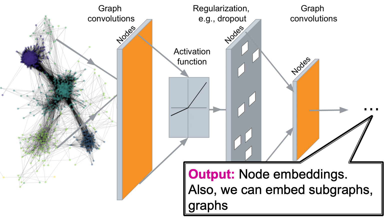
Fig. 235 Pipeline of graphical neural networks
Let
\(G\) be an undirected graph of order \(N_v\)
\(\boldsymbol{A}\) be the \(N_v \times N_v\) adjacency matrix
\(\boldsymbol{X}\) be the \(N_v \times d\) node features
A naive idea to represent the graph with features is to use the \(N_v \times (N_v + d)\) matrix \([\boldsymbol{A} , \boldsymbol{X}]\), and then feed into NN. However, there are some issues
for node-level task
\(N_v + d\) parameters > \(N_v\) examples (nodes), easy overfit
for graph-level task:
not applicable to graphs of different sizes
sensitive to node ordering
Structure
To solve the above issues, GNN borrows idea of CNN filters (hence GNN is also called graphical convolutional neural networks GCN).
Computation Graphs
In CNN, a convolutional operator can be viewed as an operator over lattices. Can we generalize it to subgraphs? How to define sliding windows?
Consider a 3 by 3 filter in CNN. We aggregate information in 9 cells and and then output one cell. In a graph, we can aggregate information in a neighborhood \(\mathscr{N} (v)\) and output one ‘node’. For instance, given messages \(h_j\) from neighbor \(j\) with weight \(w_j\), we can output new message \(\sum_{j \in \mathcal{N} (v)} w_j h_j\). In GNN, every node defines a computation graph based on its neighborhood
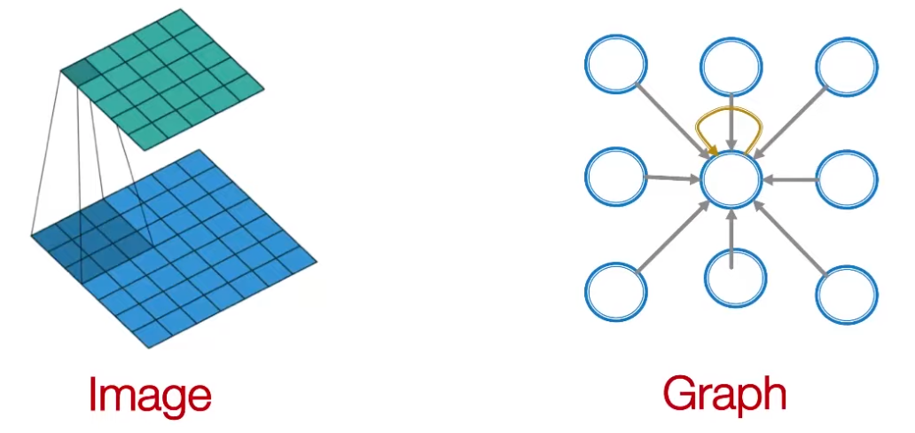
Fig. 236 CNN filter and GNN
It also borrows idea from message passing. The information in GNN propagate through neighbors like those in belief networks. The number of hops determines the number of layers of GNN. For a GNN designed to find node embeddings, the information at each layer is node embeddings.
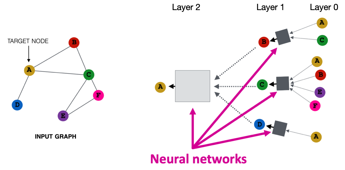
Fig. 237 Aggregation of neighbors information
Neurons
The block in the previous computation graph represents an aggregation-and-transform step, where we use neighbors’ embeddings \(\boldsymbol{h} _u ^{(\ell)}\)’s and self embedding \(\boldsymbol{h} _v ^{(\ell)}\) to obtain \(\boldsymbol{h} _v ^{(\ell + 1)}\). This step work like a neuron. Different GNN models differ in this step.
Note
One important property of aggregation is that the aggregation operator should be permutation invariant, since neighbors have no orders.
A basic approach of aggregation-and-transform is to average last layer information, take linear transformation, and then non-linear activation. Consider an \(L\)-layer GNN to obtain \(k\)-dimensional embeddings
\(\boldsymbol{h} _v ^{(0)} = \boldsymbol{x} _v\): initial \(0\)-th layer embeddings, equal to node features
\(\boldsymbol{h} _v ^{(\ell +1)} = \sigma \left( \boldsymbol{W} _\ell \frac{1}{d_v}\sum_{u \in \mathscr{N} (v)} \boldsymbol{h} _u ^ {(\ell)} + \boldsymbol{B} _\ell \boldsymbol{h} _v ^{(\ell)} \right)\) for \(\ell = \left\{ 0, \ldots, L-1 \right\}\)
average last layer (its neighbors’) hidden embeddings \(\boldsymbol{h} _u ^{(\ell)}\), linearly transformed by \(k \times k\) weight matrix \(\boldsymbol{W}_ \ell\)
also take as input its hidden embedding \(\boldsymbol{h} _v ^{(\ell)}\) at last layer (last updated embedding?? stored in \(\boldsymbol{H}\)??), linearly transformed by \(k\times k\) weight matrix \(\boldsymbol{B}_ \ell\)
finally activated by \(\sigma\).
\(\boldsymbol{z} _v = \boldsymbol{h} _v ^{(L)}\) final output embeddings.
The weight parameters in layer \(\ell\) are \(\boldsymbol{W} _\ell\) and \(\boldsymbol{B} _\ell\), which are shared across neurons in layer \(\ell\). Hence, the number of model parameters is sub-linear in \(N_v\).
If we write the hidden embeddings \(\boldsymbol{h} _v ^{(\ell)}\) as rows in a matrix \(\boldsymbol{H}^{(\ell)}\), then the aggregation step can be written as
where we update the \(v\)-th row at a neuron for node \(v\), or several rows corresponding to neurons in a layer.
In practice, \(\boldsymbol{A}\) is sparse, hence some sparse matrix multiplication can be used. But not all GNNs can be expressed in matrix form, when aggregation function is complex.
Training
Supervised
After build GNN layers, to train it, we compute loss and do SGD. The pipeline is
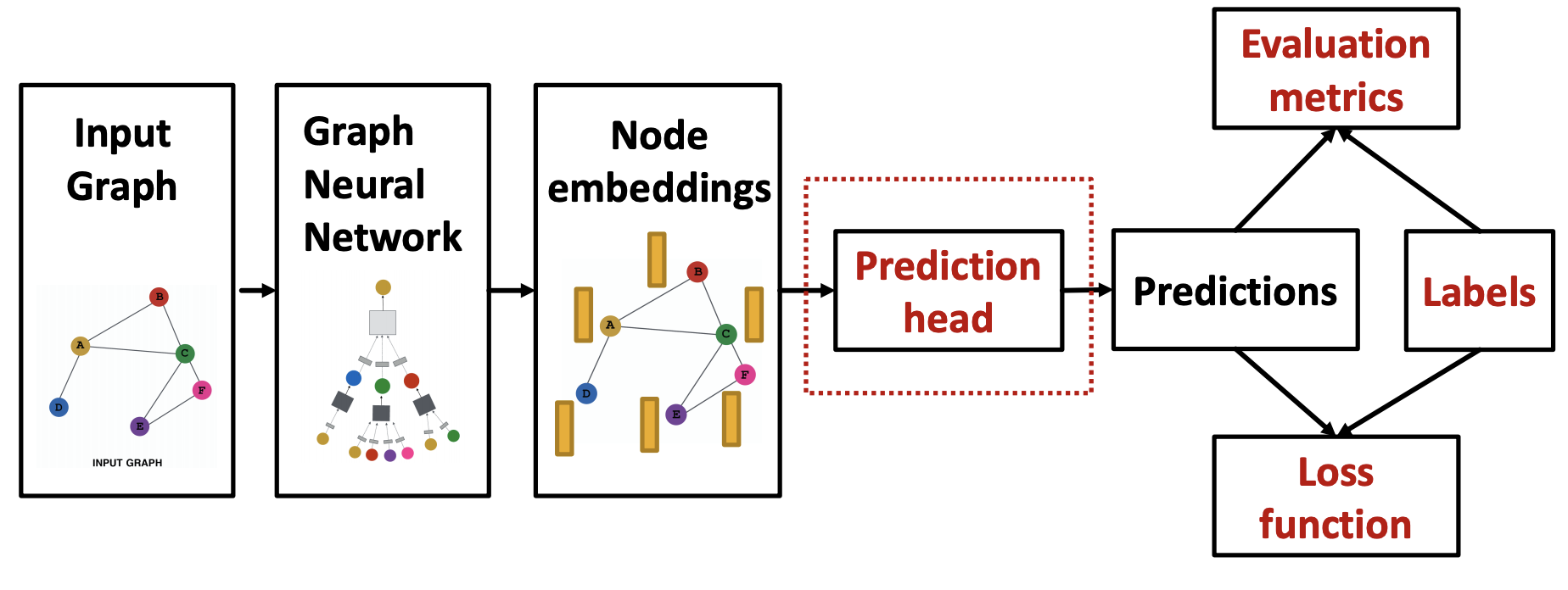
Fig. 238 GNN Training Pipeline
The prediction heads depend on whether the task is at node-level, edge-level, or graph-level.
Node-level
If we have some node label, we can minimize the loss
if \(y\) is a real number, then \(f\) maps embedding from \(\mathbb{R} ^d\) to \(\mathbb{R}\), and \(\mathcal{L}\) is L2 loss
if \(y\) is \(C\)-way categorical, \(f\) maps embedding from \(\mathbb{R} ^d\) to \(\mathbb{R} ^C\), and \(\mathcal{L}\) is cross-entropy.
Edge-level
If we have some edge label \(y_{uv}\), then the loss is
To aggregate the two embedding vectors, \(f\) can be
concatenation and then linear transformation
inner product \(\boldsymbol{z} _u ^{\top} \boldsymbol{z} _v\) (for 1-way prediction)
\(y_{uv} ^{(r)} = \boldsymbol{z} _u ^{\top} \boldsymbol{W} ^{(r)} \boldsymbol{z} _v\) then \(\hat{\boldsymbol{y}} _{uv} = [y_{uv} ^{(1)}, \ldots , y_{uv} ^{(R)}]\). The weights \(\boldsymbol{W} ^{(r)}\) are trainable.
Graph-level
For graph-level task, we make prediction using all the node embeddings in our graph. The loss is
where \(f \left( \left\{ \boldsymbol{z} _v, \forall v \in V \right\} \right)\) is similar to \(\operatorname{AGG}\) in a GNN layer
global pooling: \(f = \operatorname{max}, \operatorname{mean}, \operatorname{sum}\)
hierarchical pooling: global pooling may lose information. We can apply pooling to some subgraphs to obtain subgraph embeddings, and then pool these subgraph embeddings.
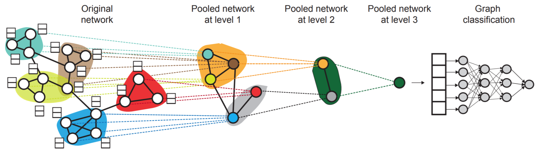
Fig. 239 Hierarchical Pooling
To decide subgraph assignment, standard community detection or graph partition algorithms can be used. The assignment can also be learned: we build two GNNs,
GNN A: one computes node embeddings
GNN B: one computes the subgraph assignment that a node belongs to
GNNs A and B at each level can be executed in parallel. See Ying et al. Hierarchical Graph Representation Learning with Differentiable Pooling, NeurIPS 2018.
Unsupervised
In unsupervised setting, we use information from the graph itself as labels.
Node-level:
some node statistics, e.g. clustering coefficient, PageRank.
if we know some nodes form a cluster, then we can treat cluster assignment as node label.
Edge-level: \(y_{u, v} = 1\) when node \(u\) and \(v\) are similar. Similarity can be defined by edges, random walks neighborhood, node proximity, etc.
Graph-level: some graph statistic, e.g. predict if two graphs are isomorphic, have similar graphlets, etc.
Batch
We also use batch gradient descent. In each iteration, we train on a set of nodes, i.e., a batch of compute graphs.
Dataset Splitting
Given a graph input with features and labels \(\boldsymbol{G} = (V, E, \boldsymbol{X} , \boldsymbol{y})\), how do we split it into train / validation / test set?
Training set: used for optimizing GNN parameters
Validation set: develop model/hyperparameters
Test set: held out until we report final performance
The speciality of graph is that nodes as observations are connected by edges, they are not independent due to message passing. Sometimes we cannot guarantee that the test set will really be held out. Some data leakage issue may exist.
Random split
In contrast to this fixed split, another way is random split: we randomly split the data set to train / validation / test. We report average performance over different random seeds.
The ways of splitting depends on tasks.
Node-level
Transductive setting: split nodes labels into \(\boldsymbol{y} _{\text{train} }, \boldsymbol{y} _{\text{valid} }, \boldsymbol{y} _{\text{test} }\).
training: use information \((V, E, \boldsymbol{X} , \boldsymbol{y} _{\text{train} })\) to train a GNN. Of course, the computation graphs are for those labeled nodes.
validation: evaluate trained GNN on validation nodes with labels \(\boldsymbol{y} _{\text{valid} }\), using all remaining information \((V, E, \boldsymbol{X})\)
test: evaluate developed GNN on test nodes with labels \(\boldsymbol{y} _{\text{test} }\), using all remaining information \((V, E, \boldsymbol{X})\)
also applicable to edge-level tasks, not applicable to graph-level tasks.
Inductive setting: partition the graph \(G\) into training subgraph \(G_{\text{train} }\), validation subgraph \(G_{\text{valid} }\), and test subgraph \(G_{\text{test} }\), remove across-subgraph edges. Then the three subgraphs are independent.
training: use \(G_{\text{train} }\) to train a GNN
valid: evaluate trained GNN on \(G_{\text{valid} }\)
test: evaluate developed GNN on \(G_{\text{test} }\)
pros: applicable to node / edge / graph tasks
cons: not applicable to small graphs
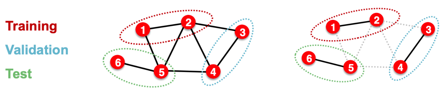
Fig. 240 Splitting graph, transductive (left) and inductive (right)
In the first layer only features not labels are fed into GNN.
Link-level
It is worth noting that a good link prediction model need to predict both existence of an edge \((a_{ij}=1)\) and non-existence of an edge \((a_{ij}=0)\), given two nodes \(i\) and \(j\). Hence, both positive edge and negative edge (non-existence) should be treated as labels. But often the graph is sparse, i.e. #negative edges >> #positive edges. Hence, negative edges are sampled in training.
In DeepSNAP, the edge_label and edge_label_index have included the negative edges (default number of negative edges is same with the number of positive edges).
Inductive setting
Partition edges \(E\) into
message edges \(E_m\), used for GNN message passing, and
supervision edges \(E_s\), use for computing objective, not fed into GNN
Partition graph into training subgraph \(G_{\text{train} }\), valid subgraph \(G_{\text{valid} }\), and test subgraph \(G_{\text{test} }\), remove across-subgraph edges. Each subgraph will have some \(E_m\) and some \(E_s\).
Training on \(G_{\text{train} }\)
Develop on \(G_{\text{valid} }\)
Test on \(G_{\text{test} }\)
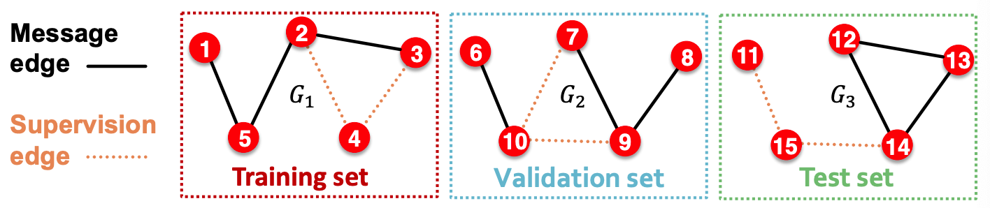
Fig. 241 Inductive splitting for link prediction
Transductive setting (common setting, edge_train_mode = "disjoint" in DeepSNAP)
Partition the edges into
training message edges \(E_{\text{train, m}}\)
training supervision edges \(E_{\text{train, s}}\)
validation edges \(E_{\text{valid}}\)
test edges \(E_{\text{test}}\)
Training: use training message edges \(E_{\text{train, m}}\) to predict training supervision edges \(E_{\text{train, s}}\)
Validation: Use \(E_{\text{train, m}}\), \(E_{\text{train, s}}\) to predict \(E_{\text{valid}}\)
Test: Use \(E_{\text{train, m}}\), \(E_{\text{train, s}}\), and \(E_{\text{valid}}\) to predict \(E_{\text{test}}\)
Another transductive setting is edge_train_mode = "all".
After training, supervision edges are known to GNN. Therefore, an ideal model should use supervision edges \(E_{\text{train, s}}\) in message passing at test time.
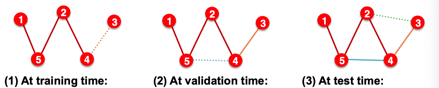
Fig. 242 Transductive splitting for link prediction
Another way of train-test split for link-prediction in general ML models:
Assume the graph have all edges labeled (no unknown edge).
Partition nodes into training set \(V_{train}\) and test set \(V_{test}\), then training set of edges \(E_{train}\) include the edges in the induced subgraph of \(V_{train}\), while test set of edges include the edges in the induced subgraph of \(V_{test}\), as well as across-subgraph edges.
\(E_{train} = E(V_{train})\)
\(E_{test} = E(V_{test}) \cup E(V_{train}, V_{test})\)
All edge sets above include both positive edges and negative edges.
Pros
Inductive capability
new graph: after training GNN on one graph, we can generalize it to an unseen graph. For instance, train on protein interaction graph from model organism A and generate embeddings on newly collected data about organism B.
new nodes: if an unseen node is added to the graph, we can directly run forward propagation to obtain its embedding.
Variants
As said, different GNN models mainly differ in the aggregation-and-transform step. Let’s write the aggregation step as
In basic GNN, the aggregation function is just average. And the update function is
This is called graph convolutional networks [Kipf and Welling ICLR 2017].
There are many variants and extensions to this update function. Before aggregation, there can be some transformation of the neighbor embeddings. The aggregation-and-transform step then becomes transform-aggregation-transform.
GraphSAGE
[Hamilton et al., NIPS 2017]
In GraphSAGE, the update function is more general,
where we concatenate two vectors instead of summation, and \(\operatorname{AGG}\) is a flexible aggregation function. L2 normalization of \(\boldsymbol{h} _v ^{(\ell + 1)}\) to a unit length embedding vector can also be applied. In some cases (not always), normalization of embedding results in performance improvement
AGG can be
Mean
\[ \operatorname{AGG} = \frac{u, v}{d_v}\sum_{u \in \mathscr{N} (v)} \boldsymbol{h} _u ^ {(\ell)} \]Pool: Transform neighbor vectors and apply symmetric vector function \(\gamma\), e.g. mean, max
\[\operatorname{AGG} = \gamma \left( \left\{ \operatorname{MLP} (\boldsymbol{h} _u ^{(\ell)} ), \forall u \in \mathscr{N} (v) \right\} \right)\]LSTM: apply LSTM, but to make it permutation invariant, we reshuffle the neighbors (some random order)
\[ \operatorname{AGG} = \operatorname{LSTM} \left( \left[ \boldsymbol{h} _u ^{(\ell)} , \forall u \in \pi (\mathscr{N} (v)) \right] \right) \]
Matrix Operations
If we use mean, then the aggregation step (ignore \(\boldsymbol{B}_\ell\)) can be written as
A variant [Kipf+ 2017]
!!Laplacian
Graph Attention Networks
If AGG is mean, then the message from neighbors are of equal importance with the same weight \(\frac{u, v}{d_v}\). Can we specify some unequal weight/attention \(\alpha_{vu}\)?
Compute attention coefficients \(e_{vu}\) across pairs of nodes \(u, v\) based on their messages, by some attention mechanism \(a\)
\[ e_{v u}=a\left(\mathbf{W}^{(l)} \mathbf{h}_{u}^{(l-1)}, \mathbf{W}^{(l)} \boldsymbol{h}_{v}^{(l-1)}\right) \]The attention coefficients \(e_{vu}\) indicates the importance of \(u\)’s message to node \(v\).
Normalize \(e_vu\) into the final attention weight \(\alpha_{vu}\) by softmax function
\[ \alpha_{v u}=\frac{\exp \left(e_{v u}\right)}{\sum_{k \in N(v)} \exp \left(e_{v k}\right)} \]
How to design attention mechanism \(a\)? For instance, \(a\) can be some MLP. The parameters in \(a\) are trained jointly.
We can generalize to use multi-head attention, which are shown to stabilizes the learning process of attention mechanism [Velickovic+ 2018]. There are \(R\) independent attention mechanisms are used. Each one of them, namely a ‘heard’, computes a set of attention weight \(\boldsymbol{\alpha} _{v} ^{(r)}\). Finally, we aggregate the \(\boldsymbol{h} _v\) again, by concatenation or summation.
\(\boldsymbol{h} _v ^{(\ell+1, \color{red}{r})} = \sigma \left( \boldsymbol{W} ^{(\ell) }\sum_{u \in \mathscr{N} (v)} \alpha_{vu}^ {(\color{red}{r})} \boldsymbol{h} _u ^ {(\ell)} \right)\)
\(\boldsymbol{h} _v ^{(\ell + 1)} = \operatorname{AGG} \left( \left\{ \boldsymbol{h} _v ^{(\ell+1, \color{red}{r})}, r = 1, \ldots, R \right\} \right)\)
Pros
allow for implicitly specifying weights
computationally efficient, parallelizable
storage efficient, total number of parameters \(\mathcal{O} (N_v + N_e)\)
If edge weights \(w_{vu}\) are given, we can
use it as weights \(\alpha_vu\), e.g. by softmax function
incorporate it into the design of attention mechanism \(a\).
In many cases, attention leads to performance gains.
GIN
Expressiveness
Consider a special case that node features are the same \(\boldsymbol{x} _{v_1} = \boldsymbol{x} _{v_2} = \ldots\), represented by colors in the discussion below. Then if the computational graph are exactly the same for two nodes, then they have the same embeddings.
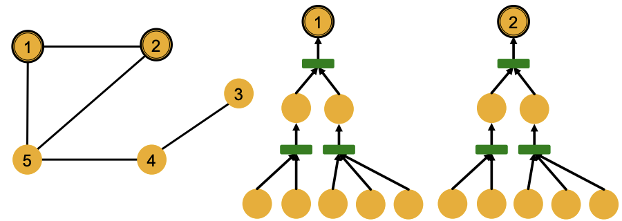
Fig. 243 Same computational graphs of two nodes
Computational graphs are identical to rooted subtree structures around each node. GNN’s node embeddings capture rooted subtree structures. Most expressive GNN maps different rooted subtrees into different node embeddings, i.e. should be like an injective function.
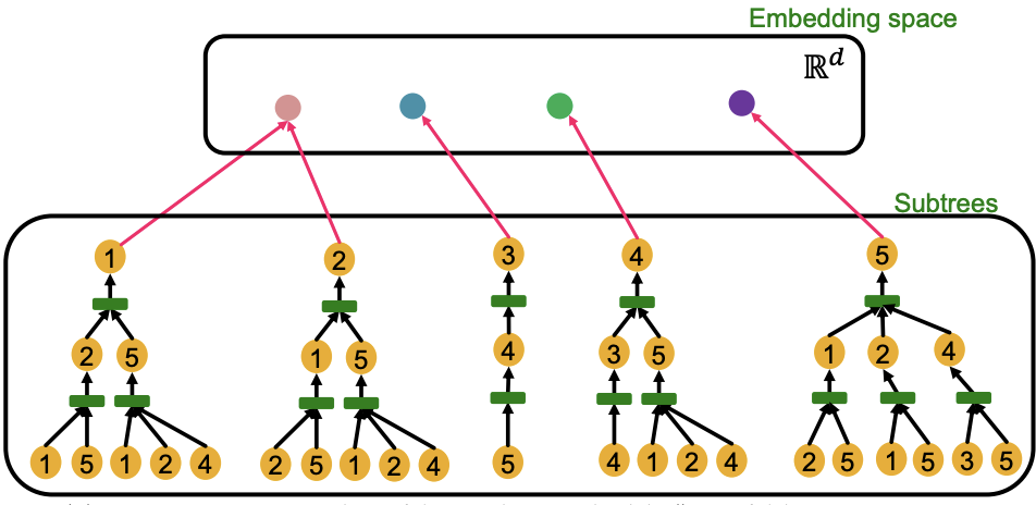
Fig. 244 Injective mapping from computational graph to embeddings
Some of the previously seen models do not use injective function at the neighbor aggregation step. Note that neighbor aggregation is a function over multi-sets (sets with repeating elements). They are not maximally powerful GNNs in terms of expressiveness.
GCN (mean-pool)
GraphSAGE aggregation function (MLP + max-pool) cannot distinguish different multi-sets with the same set of distinct colors.
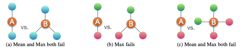
Fig. 245 Mean and max pooling failure cases
GIN
How to design maximally powerful GNNs? Can we design a neural network in the aggregation step that can model injective multi-set function.
Theorem [Xu et al. ICLR 2019]: Any injective multi-set function can be expressed as:
where \(f, \Phi\) are non-linear functions. To model them, we can use MLP which have universal approximation power.
In practice, MLP hidden dimensionality of 100 to 500 is sufficient. The model is called Graph Isomorphism Network (GIN) [Xu+ 2019].
GIN‘s neighbor aggregation function is injective. It is the most expressive GNN in the class of message-passing GNNs. The key is to use element-wise sum pooling, instead of mean-/max-pooling.
R.t. WL Kernel
It is a “neural network” version of the WL graph kernel, where the color update function is
Xu proved that any injective function over the tuple \(\left(c^{(k)}(v),\left\{c^{(k)}(u)\right\}_{u \in N(v)}\right)\) can be modeled as
where \(\varepsilon\) is a learnable scalar.
Advantages of GIN over the WL graph kernel are:
Node embeddings are low-dimensional; hence, they can capture the fine-grained similarity of different nodes.
Parameters of the update function can be learned for the downstream tasks.
Because of the relation between GIN and the WL graph kernel, their expressive is exactly the same. If two graphs can be distinguished by GIN, they can be also distinguished by the WL kernel, and vice versa. They are powerful to distinguish most of the real graphs!
Improvement
There are basic graph structures that existing GNN framework cannot distinguish, such as difference in cycles. One node in 3-node-cycle and the other in 4-node cycle have the same computational graph when layer. GNNs’ expressive power can be improved to resolve the above problem. [You et al. AAAI 2021, Li et al. NeurIPS 2020]
Layer Design
Modules
We can include modern deep learning modules that proved to be useful in many domains, including
BatchNorm to stabilize neural network training, used to normalize embeddings.
Dropout to prevent overfitting, used in linear layers \(\boldsymbol{W} _\ell \boldsymbol{h} _u ^{(\ell)}\).
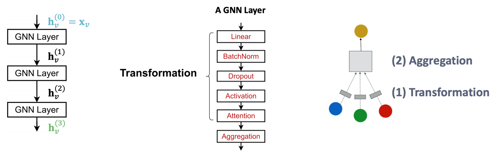
Fig. 246 A GNN Layer
Try design ideas in GraphGym.
We then introduce how to add skip connection across layers.
Issue with Deep GNN
Unlike some other NN models, adding more GNN layers do not always help. The issue of stacking many GNN layers is that GNN suffers from the over-smoothing problem, where all the node embeddings converge to the same value.
Let receptive field be the set of nodes that determine the embedding of a node of interest. In a \(L\)-layer GNN, this set is the union of \(\ell\)-hop neighborhood for \(\ell=1, 2, \ldots, L\). As the number of layers \(L\) goes large, the \(L\)-hop neighborhood increases exponentially. The receptive filed quickly covers all nodes in the graph.
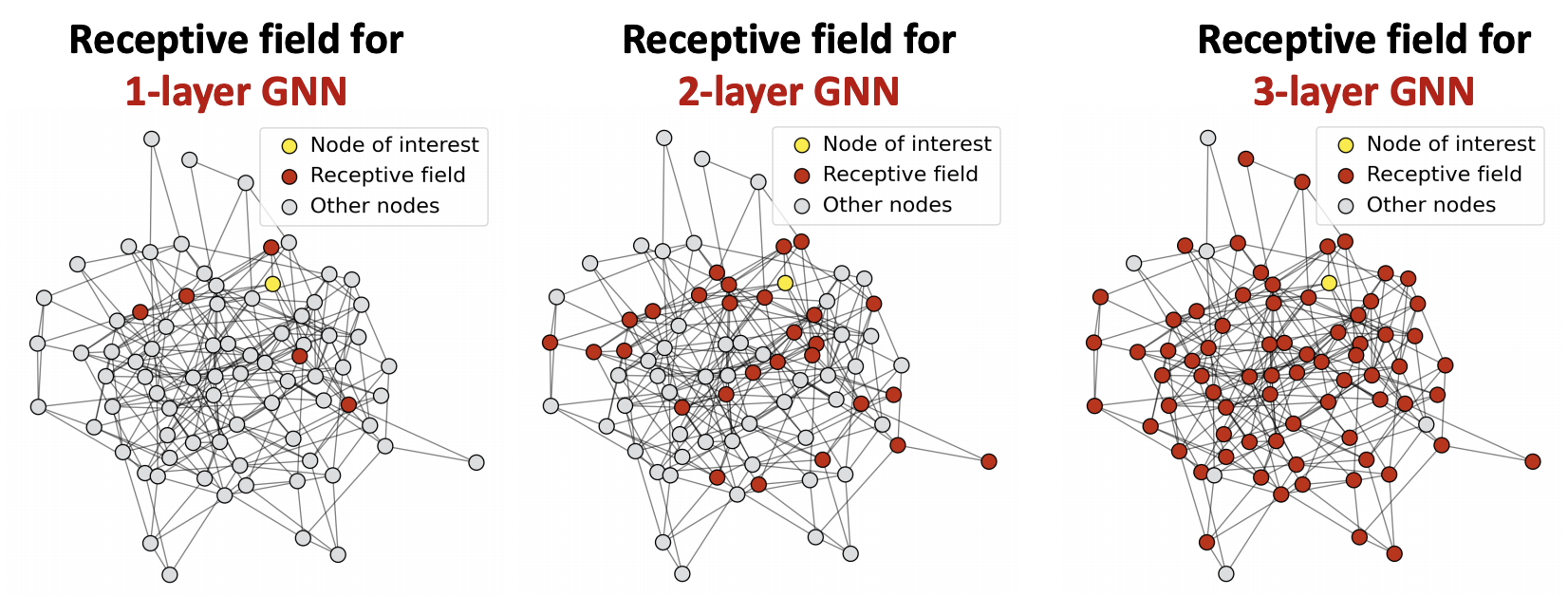
Fig. 247 Receptive field for different layers of GNN
For different nodes, the shared neighbors quickly grow when we increase the number of hops (num of GNN layers). Their computation graphs are similar, hence similar embeddings.
Solution
How to enhance the expressive power of a shallow GNN?
Increase the expressive power within each GNN layer
make \(\operatorname{AGG}\) a neural network
Add layers that do not pass messages
MLP before and after GNN layers, as pre-process layers (image, text) and post-process layers for downstream tasks.
We can also add shortcut connections (aka skip connections) in GNN. Then we automatically get a mixture of shallow GNNs and deep GNNs. We can even add shortcuts from each layer to the final layer, then final layer directly aggregates from the all the node embeddings in the previous layers
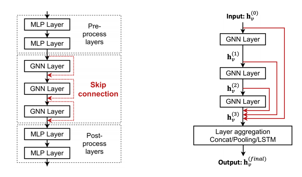
Fig. 248 Skip connection in GNN
Graph Manipulation
It is unlikely that the input graph happens to be the optimal computation graph for embeddings.
Issues and solutions:
Graph Feature manipulation
prob: the input graph lacks features.
sol: feature augmentation
Graph Structure manipulation if the graph is
too sparse
prob: inefficient message passing
sol: add virtual nodes / edges
too dense
prob: message passing is too costly
sol: sample neighbors when doing message passing
too large
prob: cannot fit the computational graph into a GPU
sol: sample subgraphs to compute embeddings
Feature Augmentation
Sometimes input graph does not have node features, e.g. we only have the adjacency matrix.
Standard approaches to augment node features
assign constant values to nodes
assign unique IDs to nodes, in the form of \(N_v\)-dimensional one-hot vectors
assign other node-level descriptive features, that are hard to learn by GNN
centrality
clustering coefficients
PageRank
cycle count (as one-hot encoding vector)
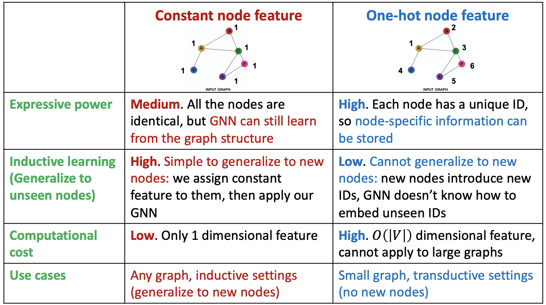
Fig. 249 Comparison of feature augmentation methods
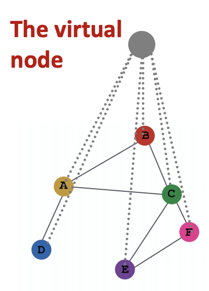
Virtual Nodes/Edges
If the graph is too sparse, then the receptive field of a node covers small number of nodes. The message passing is then inefficient. We can add virtual nodes or virtual edges to augment sparse graphs.
Virtual Edges
We can connect 2-hop neighbors via virtual edges. Rather than using adjacency matrix \(\boldsymbol{A}\), we use \(\boldsymbol{A} + \boldsymbol{A} ^2\).
For instance, in bipartite graphs, after introducing virtual edges to connect 2-hop neighbors, we obtained a folded bipartite graphs.
Neighborhood Sampling
In the standard setting, for a node \(v\), all the nodes in \(\mathscr{N} _(v)\) are used for message passing. If \(\left\vert \mathscr{N} _(v) \right\vert\) is large, we can actually randomly sample a subset of a node’s neighborhood for message passing.
Next time when we compute the embeddings, we can sample different neighbors. In expectation, we will still use all neighbors vectors.
Benefits:
greatly reduce computational cost
allow for scaling to large graphs.
Graph Generative Models
Types
Realistic graph generation: generate graphs that are similar to a given set of graphs. (our focus)
goal-directed graph generation: generate graphs that optimize given objectives/constraints, e.g. molecules chemical properties
Given a set of graph, we want to
Density estimation: model the distribution of these graphs by \(p_{\text{model} }\), hope it is close to \(p_{\text{data} }\), e.g. maximum likelihood
Sampling: sample from \(p_{\text{model} }\). A common approach is
sample from noise \(z_i \sim \mathcal{N} (0, 1)\)
transform the noise \(z_i\) via \(f\) to obtain \(x_i\), where \(f\) can be trained NN.
Challenge
large output space: \(N^2\) bits of adjacency matrix?
variable output space: how to generate graph of different sizes?
non-unique representation: for a fixed graph, its adjacency matrix has \(N_v !\) ways of representation.
dependency: existence of an edge may depend on the entire graph
GraphRNN
Recall that by chain rule, a joint distribution can be factorized as
In our case, \(x_t\) will be the \(t\)-th action (add node, add edge). The ordering of nodes is a random ordering \(\pi\). For a fixed ordering \(\pi\) of nodes, for each node, we add a sequence of edges.
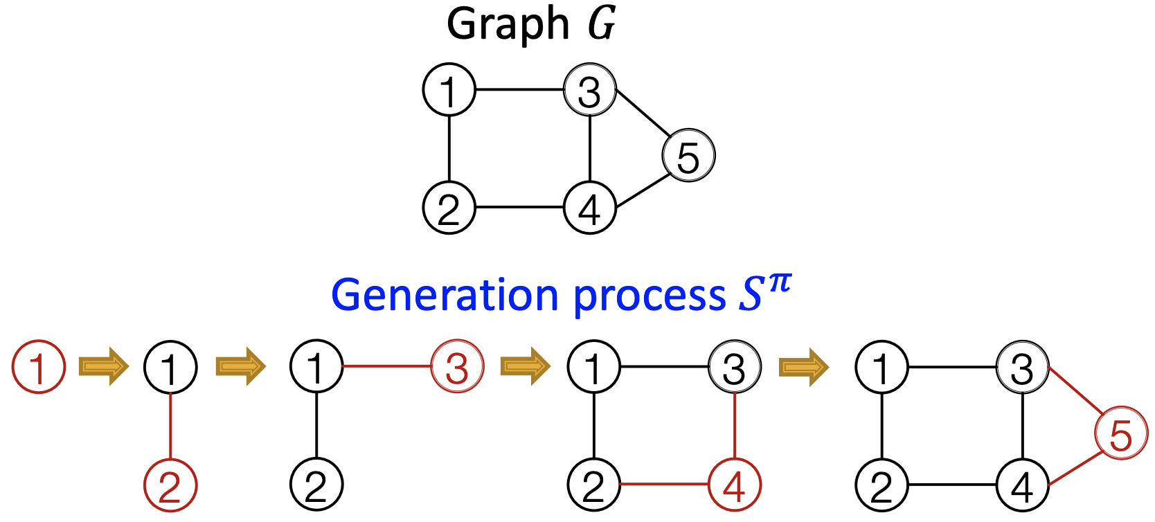
Fig. 251 Generation process of a graph
It is like propagating along columns of upper-triangularized adjacency matrix corresponding to the ordering \(\pi\). Essentially, we have transformed graph generation problem into a sequence generation problem. We need to model two processes
Generate a state for a new node (Node-level sequence)
Generate edges for the new node based on its state (Edge-level sequence)
To model these two sequences, we can use RNNs.
GraphRNN has a node-level RNN and an edge-level RNN.
Node-level RNN generates the initial state for edge-level RNN
Edge-level RNN sequentially predict the probability that the new node will connect to each of the previous node. Then the last hidden state is used to run node RNN for another step.
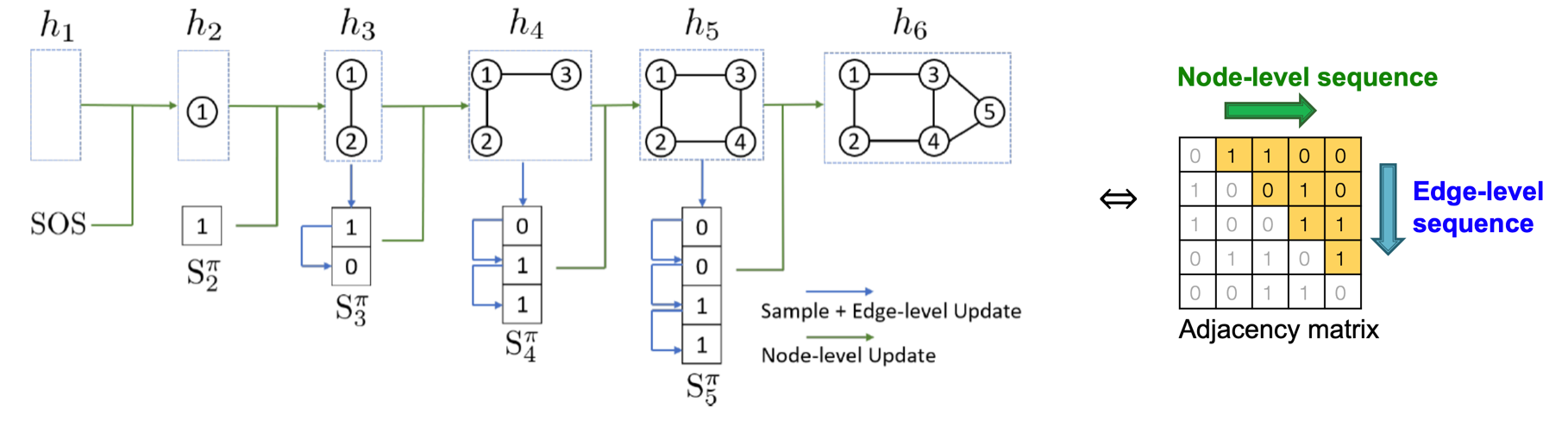
Fig. 252 GraphRNN Pipeline (node RNN + edge RNN)
The training and test pipeline is:
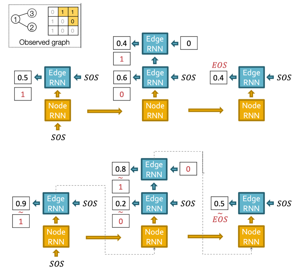
Fig. 253 GraphRNN training and test example
SOS means start of sequence, EOS means end of sequence.
If Edge RNN outputs EOS at step 1, we know no edges are connected to the new node. We stop the graph generation. At test time, this means node sequence length is not fixed.
In training of edge RNN, teacher enforcing of edge existence is applied. The loss is binary cross entropy
\[L=- \sum _{u, v} \left[y_{u, v} \log \left(\hat{y}_{u, v}\right)+\left(1-y_{u, v}\right) \log \left(1-\hat{y}_{u, v}\right)\right]\]where \(\hat{y}_{u, v}\) is predicted probability of existence of edge \((u, v)\) and \(y_{u,v}\) is ground truth 1 or 0.
Tractability
In the structure introduced above, each edge RNN can have at most \(n-1\) step. How to limit this?
The answer is to use Breadth-First search node ordering rather than random ordering of nodes.
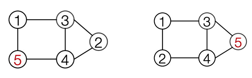
Fig. 254 Random ordering and BFS ordering
Illustrated in adjacency matrix, we only look at connectivity with nodes in the BFS frontier, rather than all previous nodes.
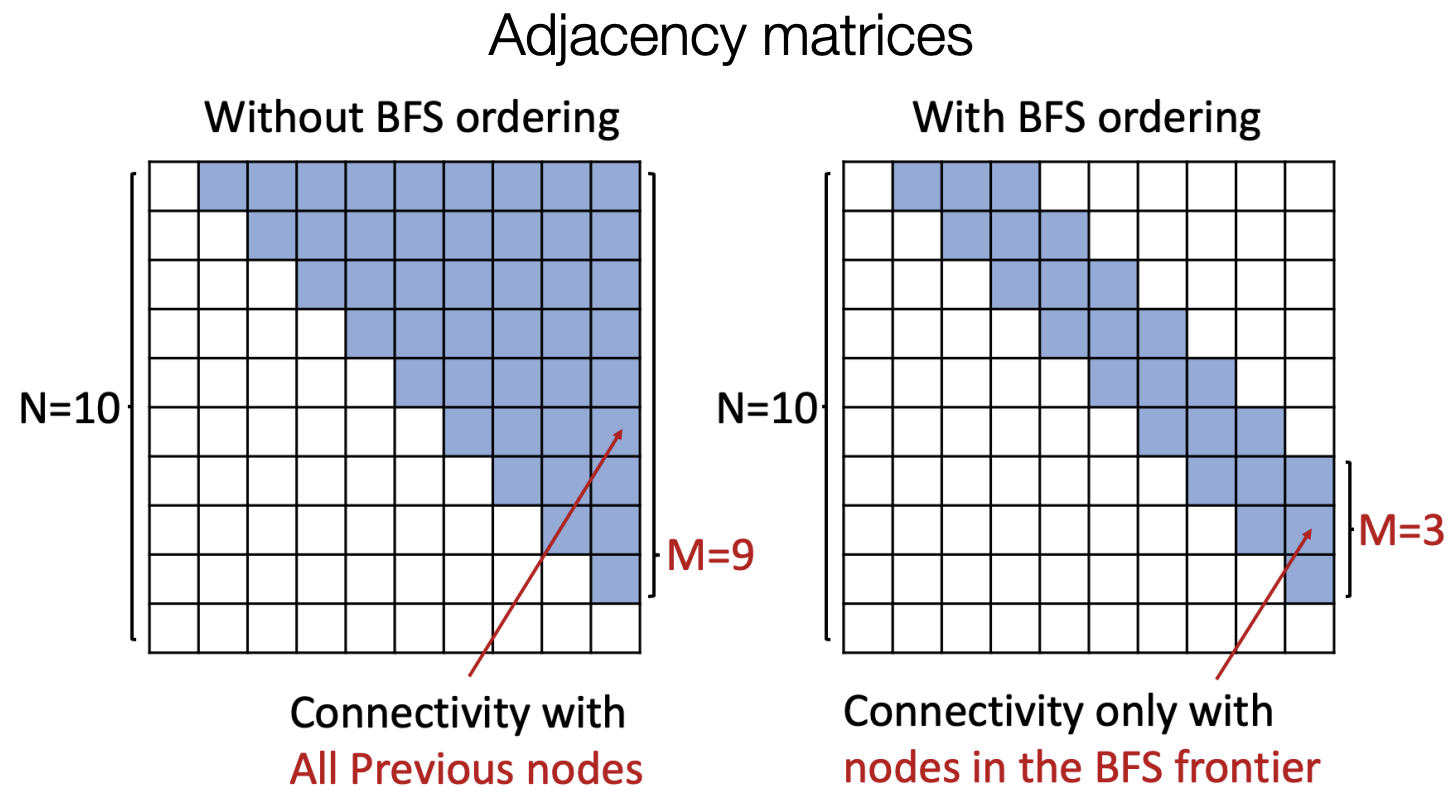
Fig. 255 Random ordering and BFS ordering in adjacency matrices
Similarity of Graphs
How to compare two graphs? Qualitatively, we can compare visual similarity. Quantitatively, we can compare graph statistics distribution such as
degree distribution
clustering coefficient distribution
Graphlet-based distribution The distance between two distributions can be measured by earth mover distance (aka Wasserstein metric in math), which measure the minimum effort that move earth from one pile to the other.
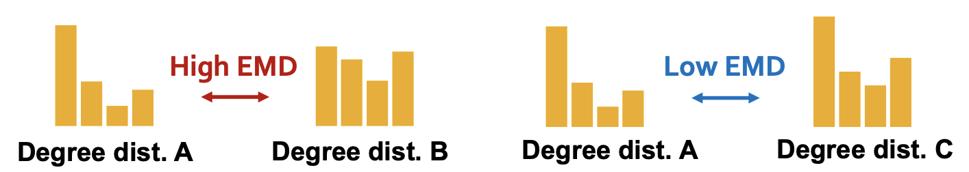
Fig. 256 Earth mover distance illustration
How two compare two sets of graphs by some set distance? Each graph element may have different \(N_v, N_e\). First we compute a statistic for each graph element, then compute Maximum Mean Discrepancy (MDD). If \(\mathcal{X} = \mathcal{H} = \mathbb{R} ^d\) and we choose \(\phi: \mathcal{X} \rightarrow \mathcal{H}\) to be \(\phi(x)=x\), then it becomes
Given a set of input graphs, we can generate a set of graphs using some algorithms. Then compare the set distance. Many algorithms are particularly designed to generate certain graphs, but GraphRNN can learn from the input and generate any types of graphs (e.g. grid).
Variants
Graph convolutional policy network
use GNN to predict the generation action
further uses RL to direct graph generation to certain goals
Hierarchical generation: generate subgraphs at each step
Limitations
For a perfect GNN:
If two nodes have the same neighborhood structure, they must have the same embedding
If two nodes have different neighborhood structure, they must have different embeddings
However,
point 1 may not be practical, sometimes we want to assign different embeddings to two nodes with the same neighborhood structure. Solution: position-aware GNNs.
point 2 often cannot be satisfied. Nodes on two rings have the same computational graphs. Sol: idendity-aware GNNs
Position-aware GNNs
J. You, R. Ying, J. Leskovec. Position-aware Graph Neural Networks, ICML 2019
structure-aware task: nodes are labeled by their structural roles in the graph
position-aware task: nodes are labeled by their positions in the graph
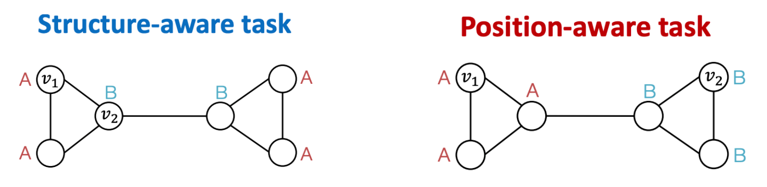
Fig. 257 Two types of labels.
GNNs differentiate nodes by their computational graphs. Thus, they often work well for structure-aware task, but fail for position-aware tasks (but node features are different??)
To solve this, we introduce anchors. Randomly pick some nodes or some set of nodes in the graph as anchor-sets. Then we compute the relative distances from every nodes to these anchor-sets.
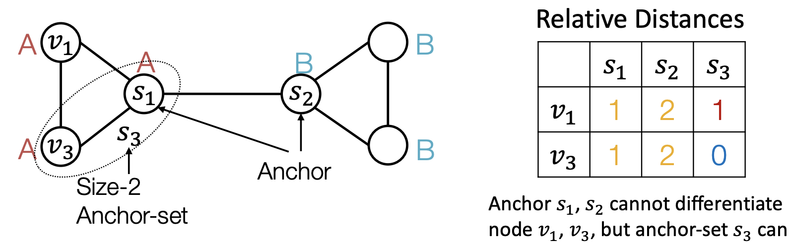
Fig. 258 Anchors
The distance can then be used as position encoding, which represent a node’s position by its distance to randomly selected anchor-set.
Note that each dimension of the position encoding is tied to an anchor-set. Permutation of the order does not change the meaning of the encoding. Thus, we cannot directly use this encoding as augmented feature.
We require a special NN that can maintain the permutation invariant property of position encoding. Permuting the input feature dimension will only result in the permutation of the output dimension, the value in each dimension won’t change.
Identity-aware GNN
[J. You, J. Gomes-Selman, R. Ying, J. Leskovec. Identity-aware Graph Neural Networks, AAAI 2021]
Heterogenous: different types of message passing is applied to different nodes. Suppose two nodes \(v_1, v_2\) have the same computational graph structure, but have different node colorings. Since we will apply different neural network for embedding computation, their embeddings will be different.
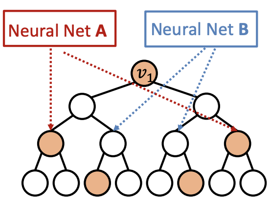
Fig. 259 Identity-aware GNN
ID-GNN can count cycles originating from a given node, but GNN cannot.
Rather than to heterogenous message passing, we can include identity information as an augmented node feature (no need to do heterogenous message passing). Use cycle counts in each layer as an augmented node feature.
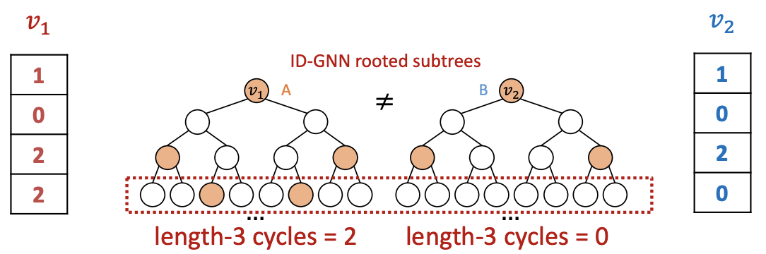
Fig. 260 Cycle count at each level forms a vector
ID-GNN is more expressive than their GNN counterparts. ID-GNN is the first message passing GNN that is more expressive than 1-WL test.
Reference
Tutorials and overviews:
Relational inductive biases and graph networks (Battaglia et al., 2018)
Representation learning on graphs: Methods and applications (Hamilton et al., 2017)
Attention-based neighborhood aggregation:
Graph attention networks (Hoshen, 2017; Velickovic et al., 2018; Liu et al., 2018)
Embedding entire graphs:
Graph neural nets with edge embeddings (Battaglia et al., 2016; Gilmer et. al., 2017)
Embedding entire graphs (Duvenaud et al., 2015; Dai et al., 2016; Li et al., 2018) and graph pooling (Ying et al., 2018, Zhang et al., 2018)
Graph generation and relational inference (You et al., 2018; Kipf et al., 2018)
How powerful are graph neural networks(Xu et al., 2017)
Embedding nodes:
Varying neighborhood: Jumping knowledge networks (Xu et al., 2018), GeniePath (Liu et al., 2018)
Position-aware GNN (You et al. 2019)
Spectral approaches to graph neural networks:
Spectral graph CNN & ChebNet (Bruna et al., 2015; Defferrard et al., 2016)
Geometric deep learning (Bronstein et al., 2017; Monti et al., 2017)
Other GNN techniques:
Pre-training Graph Neural Networks (Hu et al., 2019)
GNNExplainer: Generating Explanations for Graph Neural Networks (Ying et al., 2019)
Coding
Using PyG
In forward, GCNConv take as input both node features
xandedge_listIn training, for convenience purpose, we feed all data, but the loss only consists of
training_idx, i.e. only use training nodes to construct computation graphs, and update parametersIn validation, save the ‘best’ model with highest validation accuracy
model.train(), model.eval() flag
 binary label
out = nn.Sigmoid()    in (0, 1)
loss_fn = nn.BCELoss()  Binary Cross Entropy
los = loss_fn(out, y)
 multiple classes
out = nn.LogSoftmax(x)
loss_fn = F.nll_loss  negative log likelihood loss
loss = loss_fn(out, y)
 multiple classes
out = nn.Linear(..., data.num_classes)  raw, unnormalized scores for each class
loss_fn = nn.CrossEntropyLoss()  combines LogSoftmax and NLLLoss
loss = loss_fn(out, y)
DeepSNAP
dataset split
transformation, feature computation
Examples
Colab |
dataset |
dataset info |
task |
output |
loss |
remark |
|---|---|---|---|---|---|---|
Colab 0 |
pyg.datasets.KarateClub |
34 nodes, 34 features, 4 classes |
node classification |
|
|
only uses training set |
Colab 1 |
nx.karate_club_graph() |
embedding_dim=16, label=1 (edge) or 0 (neg edge) |
node embeddings |
|
|
convert nx graph to tensor |
Colab 2 |
Open Graph Benchmark ogbn-arxiv |
169343 nodes, 128 f |
node classification |
|
|
keep best model, no batch |
Open Graph Benchmark ogbg-molhiv |
41,127 graphs, <25> nodes, 2 classes |
graph classification |
pool |
BCEWithLogitsLoss |
AtomEncoder |
|
ENZYMES |
600 graphs, 6 classes, 3 features |
|||||
Colab 3 |
Planetoid CORA citation networks |
2708 nodes, 1433 features are elements of a bag-or-words representation of a document, 7 classes |
link prediction |
inner product |
nn.BCEWithLogitsLoss() |
Implement GraphSAGE, GAT. Loss plot. DeepSNAP |
TUDataset COX2 |
many graphs |
graph classification |
Qs
Colab 0, what are the features?
Colab 2, batch.y == batch.y? .
.
.
.
.
.
.
.