Modeling
Random Graph Models
Background
By a model for a graph we mean a collection
where
\(\mathcal{G}\) is a collection (‘ensemble’) of possible graphs
\(\mathbb{P}_\theta\) is a probability distribution on \(\mathcal{G}\)
\(\theta\) is a vector of parameters ranging over values in \(\Theta\).
Estimate \(\eta(G)\)
In traditional statistical sampling theory, there are two main approaches to constructing estimates of population parameters \(\eta(G)\) from a sample \(G^*\): design-based and model-based.
design-based: inference is based entirely on the random mechanism by which a subset of elements were selected from the population to create the sample. We have see examples in the previous section.
model-based approach: on the other hand, a model is given to specify a relationship between the sample and the population. Model-based estimation strategies including least-squares, method-of-moments, maximum-likelihood, etc are then used for constructing estimators for \(\eta(G)\).
In more recent decades, the distinction between these two approaches has become more blurred.
Assess Significance of \(\eta(G^{obs})\)
Suppose that we have a graph \(G^{obs}\) derived from observations of some sort (i.e., not necessarily through a formal network sampling mechanism). We often interested in whether \(\eta(G^{obs})\) is ‘significant’, in the sense that unusual or unexpected.
To measure this, we need a reference, like a ‘null hypothesis’ in hypothesis testing. A RGM can be used to create a reference distribution which, under the accompanying assumption of uniform likelihood of elements in \(\mathcal{G}\), takes the form,
If \(\eta(G^{obs})\) is found to be sufficiently unlikely under this distribution, this is taken as evidence against the hypothesis that Gobs is a uniform draw from \(G\).
Some issues:
How to choose \(\mathcal{G}\)?
Usually it is not possible to enumerate all elements in \(\mathcal{G}\), hence, cannot compute \(\mathbb{P}_{\eta, \mathcal{G}} (t)\) exactly \(\rightarrow\) sol: approximation.
Classical Random Graph Models
Erdos and Renyi
Equal probability on all graphs of a given order and size:
It is easy to find \(\left\vert \mathcal{G} (N_v, N_e) \right\vert = \binom{\binom{N_v}{2}}{N_e}\), hence
Gilbert
A collection \(\mathcal{G} (N_v, p)\) is defined to consist of all graphs \(G\) of order \(N_v\) that may be obtained by assigning an edge independently to each pair of distinct vertices with probability \(p\).
The level of connectivity is related to the relation between \(p\) and \(N_v\). Let \(p = \frac{c}{N}\) for \(c > 0\), then
\(c < 1\): w.h.p. all components will have \(\mathcal{O} (\log N_v)\) vertices. The largest component is a tree. No circles in the graph.
\(c > 1\): w.h.p. \(G\) will have a single connected component (‘giant component’) consisting of \(\alpha_c N_v\) vertices, for some constant \(\alpha_c > 0\), with the remaining components having only on the order of \(\mathcal{O} (\log N_v)\) vertices.
\(c > \log n\): w.h.p. \(G\) will be connected.
Fig. 210 Thresholds of exponent [Barabasi 2002]
In term of degree distribution, w.h.p.
That is, for large \(N_v\), \(G\) will have a degree distribution that is like a Poisson distribution with mean \(c = p N_v\). This is intuitive since from the perspective of a vertex \(i \in V\), it has edge \((i, j)\) w.p. \(p\) for \(N_v - 1\) number of \(j\), hence its expected degree is \(p(N_v - 1)\).
Thus, we observe
concentrated degree distribution with exponentially decay tails, rather than broad degree distribution observed in many large-scale real-world networks.
low clustering: recall that assortativity is the probability that two neighbors of a randomly chosen vertex are linked is just \(p\), which tend to zero as \(N_v\) grows.
small-world property: the diameter of the graph very like \(\mathcal{O} (\log N_v)\) w.h.p as \(N_v \rightarrow \infty\).
Reference
Generalized Random Graph Models
Equal probability on all graphs of a given order and some particular characteristic(s) \(\eta^*\):
Erdos Renyi random graph is a particular case of this, with \(\eta^* = N_e\). \(\eta^*\) can be more general, for instance, degree sequence \(\left\{d_{(1)}, \ldots, d_{\left(N_{v}\right)}\right\}\) in ordered form. Note that since \(N_v\) and \(\bar{d}\) is fixed, due to \(\bar{d} = \frac{2N_e}{N_v}\), then \(N_e\) is also fixed. Hence, they form a subset of \(\mathcal{G} (N_v, N_e)\).
Some results
suppose \(\eta\) is the first two moments of the degree distribution, under what condition will there be a giant component? [SAND 282, 283]
suppose \(\left\{ f_d \right\}\) has a power-law form \(f_d = C d^{-\alpha}\),
under what condition will there be a giant component? [SAND 5]
if \(\alpha \in (2,3)\), the diameter is \(\mathcal{O} (\log N_v)\) and average distance \(\mathcal{O} (\log \log N_v)\) w.h.p. under mild conditions [SAND 87]
if \(\alpha \in (\frac{7}{3}, 3 )\), assortativity is \(\mathcal{O} (N_v ^{- \beta})\) where \(\beta = \frac{3\alpha - 7}{\alpha - 1}\), i.e. the rate is slower than \(N_v ^{-1}\) [SAND 296.IV.B].
Simulation
Classical RGM
For some models it is actually possible to produce samples in linear time; for others, it appears that Markov chain Monte Carlo (MCMC) methods are the only realistic alternative.
\(\mathcal{G} (N_v, p)\)
A trivial solution is to store \(\binom{N_v}{2} = \mathcal{O} (N_v^2)\) independent Bernoulli random variables, each with success probability \(p\). When \(p\) is small, majority of these variables will be \(0\), hence \(\mathcal{O} (N_v^2)\) seems a waste. Can we do better? Hint: for a given vertex \(i\), consider a sequence of its \(N_v-1\) neighbors \(j\), such that \(a_{ij} \sim \operatorname{Ber}(p)\), what’s the expected number of 0’s between two 1’s?
\(\mathcal{G} (N_v, N_e)\)
It is more cumbersome to use the skipping trick above since edges are correlated: \(\sum_{i\ne j=1}^n a_{ij} = N_e\). We simply draw \(N_e\) number of distinct pairs from \((i, j) \in V^{(2)}, i\ne j\), which is a variant of coupon collector’s problem with stopping criteria of reaching \(N_e \le \binom{N_v}{2}\). This running time is \(\mathcal{O} (N_v + N_e)\) in expectation.
See Batagelj and Brandes.
Generalized RGM
Sampling GRGM is more challenging since there are more constraints. We focus our discussion upon the case that the degree sequence \(D = \left\{d_{(1)}, \ldots, d_{\left(N_{v}\right)}\right\}\) is be fixed. We introduce two algorithms with input: \(V, D\) and output: \(E\).
Matching Algorithm
create a list containing \(d_{(i)}\) copies of \(v_{(1)}\)
\[ L = \{ \underbrace{v_{(1)}, \ldots, v_{(1)}}_{d_{(1)} \text{ copies} }, v_{(2)}, \ldots, v_{(N_v)} \} \]randomly choose pairs of elements from \(L\) into \(E\), removing each pair from \(L\) once chosen.
return \(E\)
Obviously, there can be are multi-edges or loops in \(E\), hence the corresponding graph is a multi-graph. If that’s the case, just discard that graph and then repeat. Under appropriate conditions on the degree sequence, it can be argued that this algorithm will generate graphs from \(\mathcal{G}\) with equal probability. See [SAND 282].
However, when the degree distribution is skewed, e.g. \(d_{(1)}\) is large, it is quite likely to obtain repeated pairs \((v_{(1)}, v_{(j)})\) or \((v_{(1)}, v_{(1)})\). A solution is to monitor the pairs of vertices being selected and, if a candidate pair matches one in \(E\), it is rejected and another candidate pair is selected instead. This modification will introduce bias into the sampling, and the graphs \(G\) thus generated will no longer correspond to a strictly uniform sampling.
Alternatively, we can instead sample so as to avoid repeating existing matches in the first place. See [SAND 81] that developed for uniformly sampling \(r \times c\) matrices \(\boldsymbol{M}\) of non-negative integers with fixed marginal totals.
Switching Algorithm (Aka rewiring algorithms)
begin with a graph that has the prescribed degree sequence
modify the connectivity of that graph through a succession of simple changes named ‘switching’: a pair of edges in the current graph \(e_1 = (u_1, v_1)\) and \(e_2 = (u_2, v_2)\) are randomly selected and replaced by the new edges \(\left\{ u_1, v_2 \right\}\) and \(\left\{ u_2, v_1 \right\}\). If either of the latter already exists, then the proposed switch is abandoned.
It falls within the realm of MCMC methods. In practice, it is typical to let the algorithm run for some time before beginning to collect sample graphs \(G\). There is currently no theory to indicate just how long of a preliminary period is necessary. Milo et al. [SAND 279] cite empirical evidence to suggest a factor of \(100 N_e\) can be more than sufficient.
To ensure that the algorithm asymptotically yields strictly uniform sampling from \(\mathcal{G}\), there are some certain formal conditions. See [SAND 322].
MCMC can be used to generate GRG uniformly from other types of collections \(\mathcal{G}\) with additional characteristics beyond the degree sequence. However, that development of the corresponding theory, verifying the assumptions underlying Markov chain convergence, currently appears to lag far behind the pace of algorithm development.
Application
Assessing Significance
As described, given \(\eta(G^{obs})\), we want to find how in some sense unusual or unexpected it is. An important issue is determining which \(\mathcal{G}\) to use as reference. For instance, to assess the significance of the number of distinct triangles in \(G^{obs}\), a reasonable reference \(\mathcal{G}\) should have the same number of edges as that of \(G^{obs}\). In practice,
it is common to control for the degree sequence observed in \(G^{obs}\).
sometimes also control other factors: if we knew that certain groups were present within the vertex set \(V^{obs}\), we might wish to maintain the number of edges between and within each group.
For example, for an observed graph \(G^{obs}\), we find that \(\operatorname{clus}_T(G^{obs}) = 0.2257\). A reference collection \(\mathcal{G}\) can be
\(\mathcal{G} (N_v, N_e)\), or
\(\mathcal{G} (N_v, N_e, d)\), where \(d\) is the degree distribution.
Note \(\left\vert \mathcal{G} (N_v, N_e) \right\vert = \binom{\binom{N_v}{2} }{N_e}\) is quite large, and \(\left\vert \mathcal{G} (N_v, N_e, f_d) \right\vert\) is much smaller than the former but also large, we use MCMC to simulate the uniform sampling of \(10,000\) random graphs \(G\) from \(\mathcal{G}\), and compute \(\eta(G) = \operatorname{clus}_T(G)\)
in the first case, when the number of edges was fixed, only 3 of our 10,000 samples resulted in a graph with higher clustering coefficient,
whereas in the second case, when the degree distribution was fixed, all of the samples resulted in lower clustering coefficient.
We therefore have strong evidence to reject the hypothesis that the network can be viewed as a uniform sample under either random graph model. As a result, we conclude that the network graph shows markedly greater transitivity than random graphs of comparable magnitude (i.e., with respect to order and size) or connectivity (i.e., with respect to degree distribution).
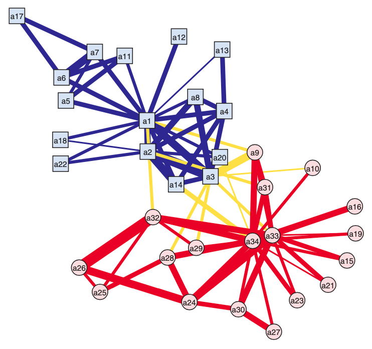
Fig. 211 Observed graph of Zachary’s ‘karate club [Kolaczyk 2009]
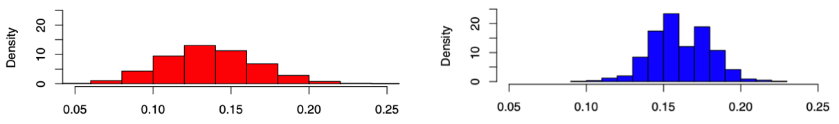
Fig. 212 Histograms of simulated clustering coefficients with fixed \(N_v, N_e\) (left) and \(f_d\) (right).
It’s also worth observing that the right distribution is bimodal.
those in in the right-hand mode tended to often be characterized by two large and somewhat distinct clusters, as in the original network.
those in the left appeared to have more diffuse clusters or even just one large cluster.
Meanwhile, for the \(\mathcal{G} (N_v, N_e, d)\) case, due to conditioning on degree, coupled with the invariance of \(\operatorname{clus} _T\) under isomorphism, the effective size of the sample space becomes quite small. In the 10,000 trials run, there were only 25 different values of \(\operatorname{clus} _T\), and 17 of them takes 99% of the mass.
Detecting Network Motifs
- Definition (motif)
Motif defined by [SAND 218, 278] are small subgraphs occurring far more frequently in a given network than in comparable random graphs.
Motivation: many large, complex networks may perhaps be constructed (at least in part) of smaller, comparatively simple ‘building blocks’. Network motif detection seeks to identify possible subgraph configurations of this nature.
Let
\(\mathcal{G} _k =\left\{ g: \left\vert V(g) \right\vert= k \right\}\) be a collection of all possible non-isomorphic \(k\)-vertex connected subgraphs.
\(L_k = \left\vert \mathcal{G} _k \right\vert\) be the cardinality
\(N_i\) be the number of occurrences of the \(i\)-th element \(g_i \in \mathcal{G} _k\) in \(G\), for \(i = 1, 2, \ldots, L_k\)
For instance, in directed graphs, when \(k=3\), \(\mathcal{G}_3\) is the collection of 13 connected subgraphs:
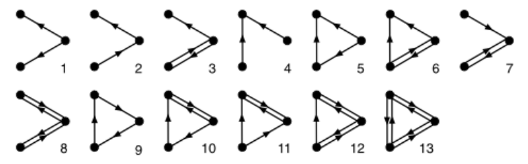
Define a proportion as our \(\eta(G)\):
Then, analogous to what was described in the previous section, each value \(F_i\) is compared to an appropriate reference distribution \(\mathbb{P}_{\mathcal{G} } (i)\). Subgraphs for whom the value \(F_i\) is found to be extreme are declared to be network motifs for building \(G^{obs}\).
Note that we for a given choice of \(k\), we need to count the number \(N_i\) for \(i = 1,\ldots, L_k\), but \(L_k\) grows quite large with \(k\). As shown above, in directed graphs, \(L_3=13\), and then \(L_4 = 199, L_5 = 9364\). To overcome this, some sampling techniques can be used. Specifically, if \(k\)-vertex subgraphs \(H\) are sampled in some fashion, then an unbiased estimate of the total number \(N_i\) of a given subgraph type is just
where \(\pi_H\) is the inclusion probability for \(H\). Natural (although biased) estimates \(\hat{F}_i\) of the corresponding relative frequencies \(F_i\) are obtained through direct substitution of \(\hat{N}_i\) to the previous equation.
For other sampling method, see SAND pg.168.
Real-world Models
Real-world graphs do not like the \(G_{n,p}\) random graphs. Many real networks have high clustering.
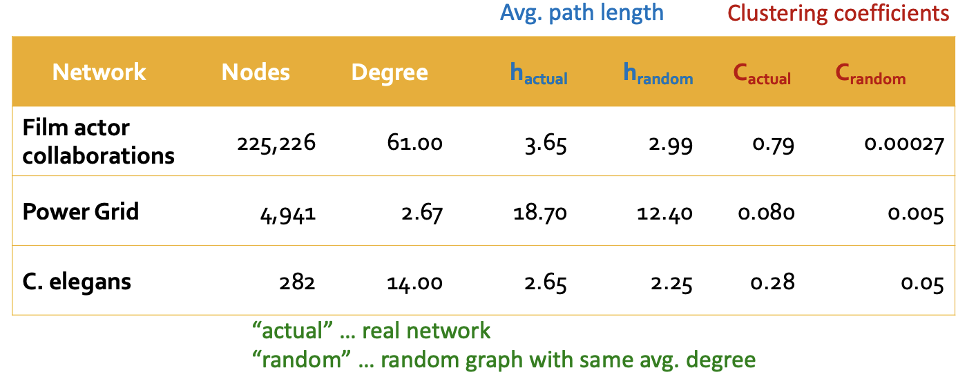
Fig. 214 Comparison of real-world graphs and random graphs with the same average degree [Leskovec 2021]
We introduce two random graph models to mimic the high clustering, high diameter properties in real-world graphs.
Note all these models (including \(G_{n, p}\)) impose prior assumption of the graph generation processes. Deep graph generative models, however, learn the graph generation process from raw data.
Small-World Models
Developed by Watts and Strogatz that mimic certain observed ‘real-world’ properties: high levels of clustering, but small distances between most nodes.
To model this, consider starting with a lattice, and randomly rewiring a a few edges. Specifically,
begin with a set of \(N_v\) vertices, arranged in a ‘ring’-like fashion
join each vertex to a \(r\) of its neighbors to each side.
for each edge, w.p. \(p\), independently move one of its end to be incident to another uniformly randomly chosen vertex, but avoid loops and multi-edges.
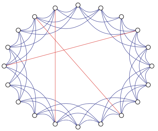
Fig. 215 Example of a Watts-Strogatz ‘small-world’ network graph. [Kolaczyk 2009]
For a lattice \(G\) with parameter \(r\) described above, it is easy to find
high level of clustering: \(\operatorname{clus}_T (G) = \frac{3r-3}{4r-2} \approx \frac{3}{4}\)
long diameter: \(\operatorname{diam}(G) = \frac{N_v}{2r}\)
long average distance: \(\bar{l} = \frac{N_v}{4r}\)
But, addition of a few randomly rewired edges has the effect of producing ‘short-cuts’ in the graph, but it takes a lot of randomness to ruin clustering. In numerical simulation shown below, after rewiring with some small \(p\), we have \(\bar{l} = \mathcal{O} (\log N_v)\) while keep clustering coefficient close to \(\frac{3}{4}\).
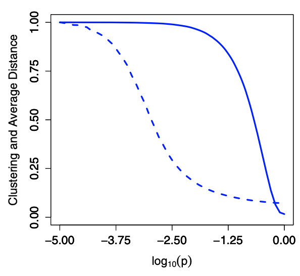
Fig. 216 Simulation results of clustering coefficient \(\operatorname{clus}(G)\) (solid) and \(\bar{l}\) (dashed) as a function of \(p\), both have been normalized by their largest values
Essentially, it interpolate between regular lattice graphs and \(G_{n,p}\) random graph.
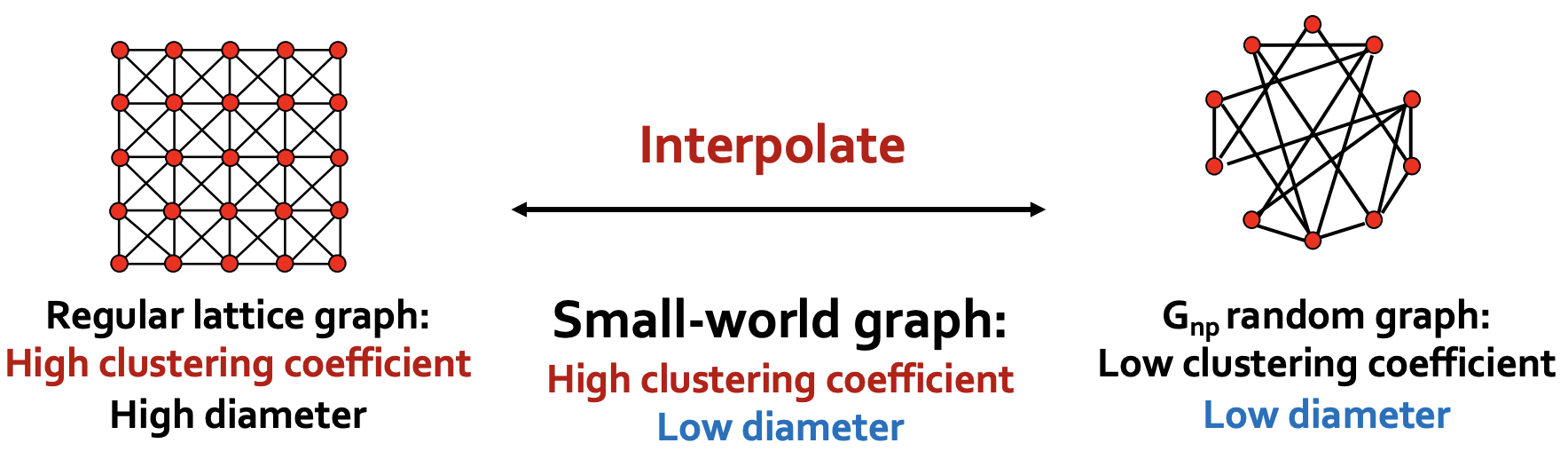
Fig. 217 Small world model as interpolation [Leskovec 2021]
However, the closed form for \(\operatorname{clus}(G)\) and \(\bar{l}\) are still open problems.
Variation:
both ends of an edge are rewired [SAND 23]
no edges are rewired, but some small number of new edges are added to randomly selected pairs of vertices [SAND 284, 298]
add edge \((u, v)\) w.p. inversely proportional to \(\operatorname{dist} (u,v)\), i.e. \(p \propto (\operatorname{dist} )^{-r}\) for some \(r > 0\). [SAND 229, 231].
Kronecker Graph Model
Kronecker product \(\otimes\) is a way of generating self-similar matrices. It is defined as
If \(\boldsymbol{A}, \boldsymbol{B}\) are the adjacency matrix of a graph, then Kronecker power mimics recursive graph/community growth.
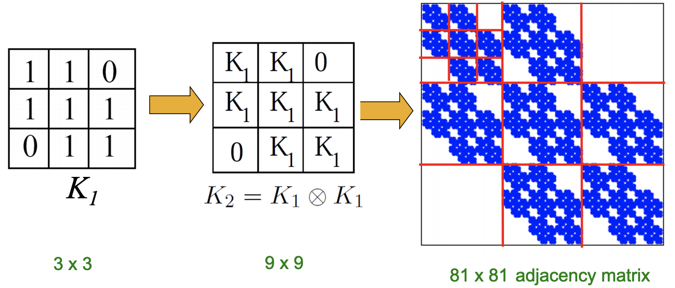
Fig. 218 Kronecker power of a adjacency matrix [Leskovec 2021]
Kronecker graph model uses it to construct a random matrix with Bernoulli matrix.
Create \(N_1 \times N_1\) probability matrix \(\boldsymbol{\Theta}_1\), where all entry values are in \((0, 1)\).
Compute the \(k\)-th Kronecker power \(\boldsymbol{\Theta}_k\).
For each entry \(p_{uv}\) in matrix \(\boldsymbol{\Theta}_k\), include an edge \((u, v)\) with probability \(p_{uv}\).
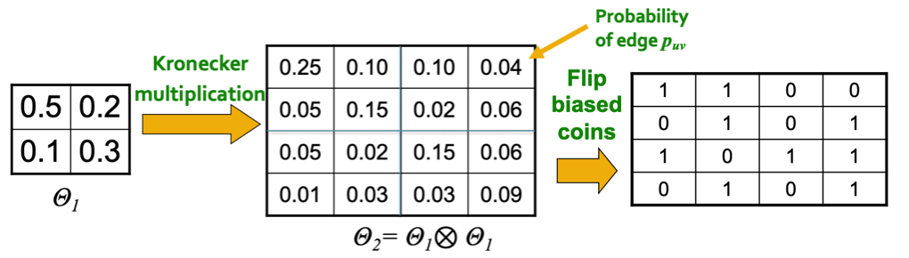
Fig. 219 Adjacency matrix in Kronecker graph models [Leskovec 2021]
Obviously, there involves \(\mathcal{O} (N_v^2)\) Bernoulli random variables. To improve this, we can exploit the recursive structure of Kronecker graphs.
It is quite close to real graphs.
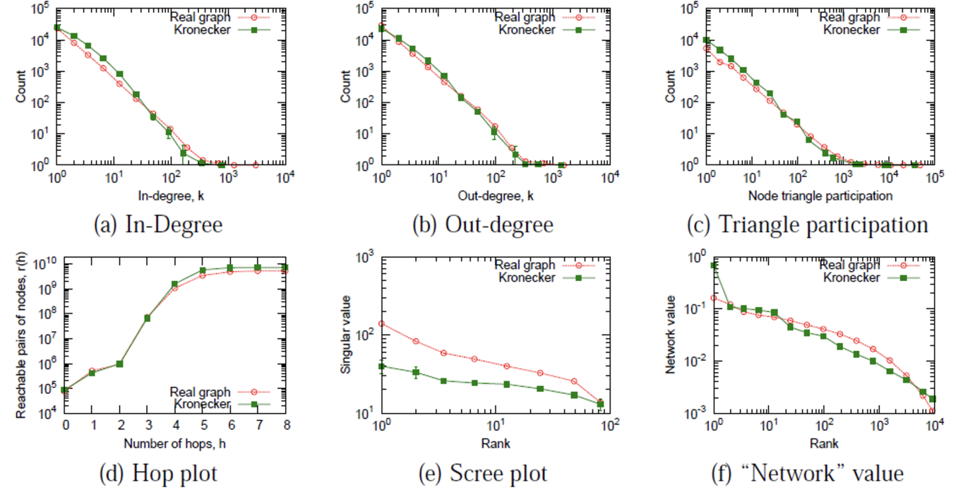
Fig. 220 A Kronecker graph vs a real graph [Leskovec 2021]
Growth Models
Many networks grow or otherwise evolve in time, e.g. WWW and citation networks. Problems of interest include
how the graph changes? how to model?
vertex preference, fitness, copying, etc
as \(t\) goes large, some properties emerge
Preferential Attachment
principle: the rich get richer.
observe: in WWW, often web pages to which many other pages point will tend to accumulate increasingly greater numbers of links as time goes on.
want to mimic: broad degree distributions, as observed in many large, real-world networks
We introduce Barabasi-Albert Model, which view degree as ‘richness’.
Start with an initial graph \(G{(0)}\) of \(N(0)_v\) vertices and \(N^{(0)}_e\) edges.
At stage \(t = 1,2, \ldots\), the current graph \(G^{(t−1)}\) is modified to create a new graph \(G^{t}\) by
adding a new vertex of degree \(m\ge 1\), where the \(m\) new edges are attached to \(m\) different vertices in \(G^{(t−1)}\), with probability \(\frac{d_v}{\sum_{v ^\prime \in V} d_{v ^\prime}}\) for \(v\) to be connected (preferential to those with higher degrees).
\(G^{t}\) will have \(N_v^{(t)} = N_v^{(0)} + t\) vertices and \(N_e^{(t)} = N_e^{(0)} + tm\) edges
We would expect that a number of vertices of comparatively high degree (“rich”) should gradually emerge as \(t\) increases.
How to select \(m\) vertices exactly? We introduce the linearized-chord diagram (LCD) model. For simulation of LCD in linear time, see [SAND 23].
For the case \(m=1\),
begin with \(G^{(1)}\) consisting of a single vertex with a loop
for \(t = 2, 3 \ldots,\)
add the vertex \(v_t\) to \(G^{(t-1)}\) with an edge to a vertex \(v_s\) for \(1 \le s \le t\) chosen randomly w.p.
\[\begin{split} \mathbb{P}(s=j)=\left\{\begin{array}{ll} d_{G(t-1)}\left(v_{j}\right) /(2 t-1), & \text { if } 1 \leq j \leq t-1 , \\ 1 /(2 t-1), & \text { if } j=t, \end{array}\right. \end{split}\]where \(d_{G^{(t-1)}}\left(v_{j}\right)\) is the degree of \(v_j\) at time \(t-1\).
For the case \(m > 1\), we repeat the above process for \(m\) steps, after which we contract the added \(m\) vertices into one, with the \(m\) edges retained. Clearly, this formulation allows for loops and multi-edges. However, these should occur relatively rarely, and the precision gained by this formulation is necessary for rigorously deriving mathematical results regarding model properties for \(G^{(t)}\):
connected w.h.p. (not connected if, e.g., \(m=1, j=t\) self-loop).
power-law degree w.h.p. \(t\) tends to infinity, \(G^{(t)}\) have degree distributions that tend to a power-law form \(d^{-\alpha}\) with \(\alpha = 3\). It can be shown that w.h.p. for any \(\epsilon\) and every \(0 \le d\le \left(N_{v}^{(t)}\right)^{1 / 5}\),
\[ f_{d}\left(G^{(t)}\right) \in (1 \pm \varepsilon) f_{d, m} \quad \text{where } f_{d, m}= \frac{2m(m+1)}{(d+2)(d+1) d} \]which behaves like \(d^{-3}\) for \(d\) large relative to \(m\).
small diameter: when \(m=1\), diameter \(\operatorname{diam}(G^{(t)}) = \mathcal{O} (\log N_v^{(t)})\). when \(m>1\), it is \(\mathcal{O} \left( \frac{\log N_v^{(t)}}{\log \log N_v^{(t)}} \right)\), which is a bit smaller still.
less clustering
\[ \mathbb{E} [\operatorname{clus}_T (G^{(t)}) ] = \mathcal{O} \left( \frac{m-1}{8} \frac{\left(\log N_{v}^{(t)}\right)^{2}}{N_{v}^{(t)}} \right) \]which is only a little better than \(N_v^{-1}\) behavior in the case of classical random graph models.
There many extensions and variations, such as
clustering, diameter, etc
consider other ‘fitness’ or inherent quality of vertices as ‘richness’?
allow \(m\) to vary, or dynamic addition and removal of edges?
add offset \(d^*\) to \(d_v + d^*\), or use powers \(d_v^\gamma\).
The main concern include
whether or not a power-law limiting distribution is achieved?
if so, how is \(\alpha\) related to model parameters?
See [SAND 6, 296, 41].
Copying Models
Copying model is distinct from preferential attachment but can also produce power-law degree distributions.
Full Copying
Chung, Lu, Dewey, and Galas [SAND 89]
beginning with an initial graph \(G^{(0)}\),
for \(t = 1, \ldots,\)
choose a vertex \(u\) from graph \(g^{(t)}\)
add a new vertex \(v\), join it with each of the neighbors of \(u\) independently w.p. \(p\)
The degree distribution \(f_d{G ^{(t)} }\) will tend to a power-law form \(d^{-\alpha}\) w.h.p,, where \(\alpha\) satisfying
This equation will have two solutions \(\alpha\) for any given \(p\), but only one will be stable.
For \(p > 0.5671 \ldots\), the stable solution is \(\alpha = 1\)
For \(p=1/2\), it is \(\alpha = 2\)
For \(p=1\), no power-law behavior. To achieve power-law, it is sufficient to allow partial duplication to occur some fraction \(q \in (0,1)\) of the times.
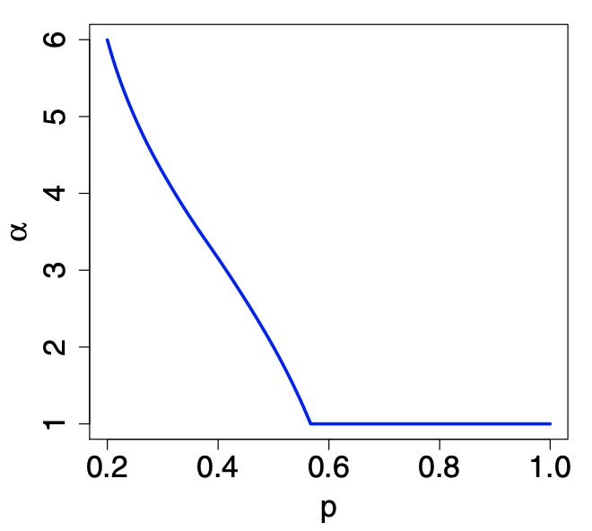
Fig. 221 Power-law exponent \(\alpha\) as a function of \(p\) in copying model. [Kolaczyk 2009]
Partial Copying
Kleinberg et al. [SAND 232] and by Kumar et al. [SAND 241]
for \(i=1, \ldots, m\), w.p. \(1-\beta\) copying the \(i\)-th neighbor of \(u\), and w.p. \(\beta\) to form edge between \(v\) and some vertex uniformly selected from \(G^{(t-1)}\). [SAND 232 241].
Intuition
In WWW, when an individual setting up a new web page,
On the one hand, the web page is likely being set up in the context of some established topic(s), and thus will probably include a number of established links in that topic.
On the other hand, an individual also brings their own perspective to the topic, and will be expected to generate some previously unseen links as well
In protein interaction networks, structure of genes associated with the proteins as typically evolving through duplication, as above, but periodically arising instead through mutation.
Properties
The degree distribution \(\left\{ f_d(G ^{(t)} ) \right\}\) also tends to a power law. For each \(d >0\), as \(t \rightarrow \infty\),
\[ f_{d} \rightarrow f_{0} \prod_{j=1}^{d} \frac{1+\beta /(j(1-\beta))}{1+2 /(j(1-\beta))} \]which behave like \(d ^{-\alpha}\) for \(\alpha = \frac{2-\beta}{1-\beta}\).
generates many more dense bipartite subgraphs than are found in comparable classical random graphs, which is encountered in real web graphs.
Fitting
We need to observe how the graph change over time, i.e. a sequence of ‘snap-shots’ of the graph. But often we only have the final shot. In this situation, we can still do fitting. See [SAND 407] which makes clever usage of their recursive nature to get around this lack of multiple snap-shots.
Exponential Random Graph Models
ERGM are better than the above models, in construction, estimation, comparison etc.
Consider a random graph \(G = (V, E)\), let \(\boldsymbol{Y}\) be the random adjacency matrix. An ERGM is a model specified in exponential family form for the joint distribution of the elements \(y_{ij}\):
where
each \(H\) is a configuration: a set of possible edges among a subset of the vertices in \(G\)
\(g_{H}(\boldsymbol{y})=\prod_{y_{i j} \in H} y_{i j}\), which is \(1\) if the configuration \(H\) occurs in \(\boldsymbol{y}\), or \(0\) otherwise.
a non-zero value for \(\theta_H\) means that the \(Y_{ij}\) are independent in \(H\), conditional upon the rest of the graph
\(\kappa = \kappa(\theta)=\sum_{\boldsymbol{y}} \exp \left\{\sum_{H} \theta_{H} g_{H}(\boldsymbol{y})\right\}\) is a normalization constant.
Note that
The summation implies a certain (in)dependency structure among \(Y_{ij}\). For given index set \(\mathcal{A}, \mathcal{B}, \mathcal{C}\), the random variables \(\left\{ Y_{i, j} \right\}_{(i, j) \in \mathcal{A}}\) and independent of \(\left\{ Y_{i, j} \right\}_{(i, j) \in \mathcal{B}}\), given the values of \(\left\{ Y_{i, j} \right\}_{(i, j) \in \mathcal{C}}\).
Conversely, we can begin with a collection of (in)dependence relations among subsets of elements in \(\boldsymbol{Y}\) and try to develop a model. But certain conditions need to be satisfied, that are formalized in the Hammersley-Clifford theorem [SAND 36].
One nice property:
\[ \log \left[\frac{\mathbb{P}_{\theta}\left(Y_{i j}=1 \mid \boldsymbol{Y}_{(-i j)}=\boldsymbol{y}_{(-i j)}\right)}{\mathbb{P}_{\theta}\left(Y_{i j}=0 \mid \boldsymbol{Y}_{(-i j)}=\boldsymbol{y}_{(-i j)}\right)}\right]=\theta^{\top} \Delta_{i j}(\boldsymbol{y}) \]
Bernoulli Random Graphs
If we assume each edge \(e(i, j)\) is formed independently with probability \(p_{ij}\), i.e. \(y_{ij} \sim \operatorname{Ber}(p_{ij})\) and \(y_{i,j} \perp y_{i ^\prime , j ^\prime}\) for any \((i, j)\ne (i ^\prime , j ^\prime)\), then
\(\theta_H = 0\) for all configurations \(H\) involving three or more vertices.
\(g_H(\boldsymbol{y}) = g_{ij}(\boldsymbol{y}) = y_{ij}\).
The ERGM model reduces to
which is another way of writing \(p_{ij} = \frac{\exp(\theta_{ij})}{1+\exp(\theta_{ij})}\).
Obviously, this is \(\mathcal{O} (N_v^2)\) number of parameters. It is common to impose an assumption of homogeneity across vertex pairs, e.g. \(\theta_{ij} \equiv \theta\) for all \((i, j)\). Hence
which is exactly the random graph model \(\mathcal{G} (N_v, p)\) with \(p = \frac{\exp(\theta)}{\exp(\theta)}\).
More generally, we can consider a partition of two sets \((S_1, S_2)\) of vertices, and impose homogeneity within and between sets, i.e. 3 kinds of \(\theta\) values. The model is then
where \(L_{11}(\boldsymbol{y})\) and \(L_{22}(\boldsymbol{y})\) are the number within-set edges for \(S_1\) and \(S_2\) respectively, and \(L_{12}(\boldsymbol{y})\) is the number of across-set edges.
Cons
assumption of complete independence is untenable in practice
Bernoulli-like random graphs lack many characteristics of real-world graphs
Markov Random Graphs
[SAND 155]
Markov dependence: two possible edges are dependent whenever they share a vertex, conditional on all other possible edges. That is, the presence or absence of \((i, j)\) depends on that of \((i, k)\) for \(k\ne j\), given information on all other edges. A random graph G arising under Markov dependence conditions is called a Markov graph.
What’s the joint distribution? Using the Hammersley-Clifford theorem, \(G\) is a Markov graph if and only if the joint distribution can be expressed as
where
\(S_1(\boldsymbol{y} )=N_e\)
\(S_k(\boldsymbol{y})\) is the number of \(k\)-stars (a tree with one vertex of degree \(k\) and \(k\) neighbors of degree 1).
\(T(\boldsymbol{y})\) is the number of triangles
Note that
the statistics \(S_k\) and \(S_{k ^\prime}\) are expected to be correlated (\(k\) stars implies \(k ^\prime\)-stars for \(k ^\prime < k\))
\(S_k\) and \(T\) are also correlated
fitting higher order of \(k\) is hard
Fitting
The MLEs \(\hat{\theta}_H\) of \(\theta_H\) are well defined but the calculation is non-trivial. There is no developed theory for CI, testing, due to the highly dependent nature of observations.
The log-likelihood is
where \(\psi(\theta) = \log \kappa (\theta)\) and \(\kappa(\theta)=\sum_{\boldsymbol{y}} \exp \left\{\theta^{\top} \boldsymbol{g}(\boldsymbol{y})\right\}\). Taking derivative w.r.t. \(\theta\) on both sides gives
Note the fact \(\mathbb{E}_{\theta}[\boldsymbol{g}(\boldsymbol{Y})]=\partial \psi(\theta) / \partial \theta\). Hence the MLE can be expressed as the solution to the system of equations
Approximate Log-likelihood
However, \(\psi(\theta)\) is hard to evaluate since it involves \(\sum_{\boldsymbol{y}}\) over \(2^{\binom{N_v}{2} }\) possible choice of \(\boldsymbol{y}\), for each \(\theta\). Two Monte Carlo approaches are used
stochastic approximation of the log-likelihood \(\ell(\boldsymbol{\theta} )\) [SAND 209]
stochastic approximation to solutions of systems of equations \(\boldsymbol{g}(\boldsymbol{y}) = \frac{\partial \psi(\theta)}{\partial \theta}\) by Robbins-Monro algorithm [SAND 324].
Log-pseudo-likelihood
A disadvantage of both of the methods above is their computationally intensive nature. To date they have been applied to networks with at most a few thousand vertices. An alternative is to estimate \(\theta\) by maximizing the log-pseudo-likelihood
pros
work best when dependencies among the elements of \(\boldsymbol{y}\) are relatively weak.
computationally expedient
cons
the above condition does not hold in many real-world contexts
See [SAND 37, 372]
Goodness-of-fit
Still not well developed for graph modeling contexts. Some practice steps are
simulate numerous random graphs from the fitted model
compare high-level summary characteristics of these graphs, with those of the originally observed graph
if poor match, then this suggests systematic differences between the specified class of models and the data, i.e. lack of goodness-of-fit
Model Degeneracy
- Definition (Model degeneracy)
a probability distribution that places a disproportionately large amount of its mass on a correspondingly small set of outcomes.
For instance, a number of simple but popular Markov graph models have been shown to be degenerate: places most of its mass on either the empty graph, the complete graph, or a mixture of the two, depending on the value of \(\theta\).
For degenerate models, the transition boundary (from empty, to mixture, to complete) of \(\theta\) is sharp. As a result, for poorly specified ERGMs, numerical algorithms like MCMC can have substantial difficulty converging.
For a case study see [SAND pg.188].
Challenges
How to incorporate our understanding of working of an underlying complex system into the model?
inference
model specification
Related topics
dynamical/complex systems
agent-based modeling (economics, sociology)
graphical models