Fourier Transform-based Representations¶

Why study Fourier transform in ML?

Staple of feature representation for many types of data (audio, images, others) for many decades, still useful in many settings
Also useful for deriving new algorithms in machine learning

Before we do any learning, we start with some data representation. Typically, this involves converting raw data into feature vectors. These days, much of feature engineering is replaced by neural network-based feature learning. But not all…choice of initial representation can still be important for

Visualization of raw data
Qualitative understanding of the data
Better input to a learning algorithm
When number of observations is small, handcraft features are also useful than complicated models, e.g. neural networks

Fourier methods include

Discrete-time and continuous-time Fourier series
Discrete-time and continuous-time Fourier transforms
Discrete Fourier transform (most common for digital signals)

Basics¶

Main idea¶

Decompose a signal \(\left\{ \boldsymbol{x} _t \right\}=x_0, x_1, \ldots, x_{N-1}\) as a sum of multiple sinusoids at different frequencies

\[x_t=\sum_{k} a_{k} f_{k}(t)\]

where

Signal = function of a discrete “time” variable \(n\)
Subscript notation reminds us that the time variable is discrete
\(f_k(t)\) sinusoid (sine/cosine function) at frequency indexed by \(k\)
\(a_k =\) “amount” of frequency \(k\) present in \(\left\{ \boldsymbol{x} _t \right\}\), aka “spectrum” of the signal (but this word has other meanings).
Fourier transform algorithms: ways of finding \(a_k\) given \(\left\{ \boldsymbol{x} _t \right\}\)

Demo:

http://www.falstad.com/dfilter/
https://www.youtube.com/watch?v=spUNpyF58BY&ab_channel=3Blue1Brown

Motivation¶

Physiology of hearing suggest that the structure of human ears are doing Fourier transform.

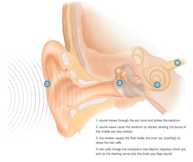
Fig. 56 Hairs in the cochlea (3) have different frequency responses [image link]¶

Examples and Applications¶

Speech

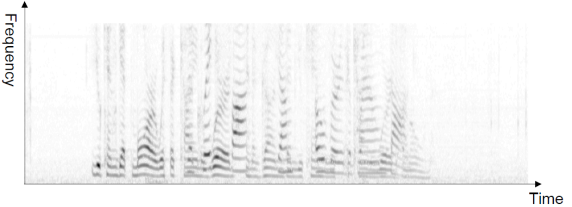
Fig. 57 Separate components from a speech (apply FT to rolling windows)¶
Financial market data
Weather data
Medical imaging, other scientific imaging
Image compression (e.g. JPEG)

Applications to machine learning

Feature extraction, compression and de-noising of speech/images: Can be an important precursor to unsupervised (or supervised) learning
Approximating kernels [Rahimi & Recht 2007]
Speeding up convolutional neural networks [Mathieu et al. 2013]
Analyzing and regularizating neural networks [Aghazadeh et al. 2020]

Discrete Fourier Transform (DFT)¶

We often start with a very long signal and compute its spectrum over sub-sequences (“windows”) of fixed length \(N\) starting at sample \(t\)

\[ \left\{ \boldsymbol{x}_t \right\} = x_t, x_{t+1}, \ldots x_{t+N-1} \]

Transformation¶

The discrete Fourier transform (DFT) transforms \(\left\{ \boldsymbol{x}_t \right\}\) into another sequence \(\left\{ \boldsymbol{X} _k \right\} = X_0, X_1, \ldots, X_{N-1}\) where

\[ X_k=\sum_{n=t}^{t+N-1} x_n e^{-j 2 \pi k n / N}, \quad k=0, \ldots, N-1 \]

The DFT \(\left\{ \boldsymbol{X} _k \right\}\) is also called the spectrum. \(X_k\) is the value of the spectrum at the \(k\)-th frequency
Equivalently, we can consider \(k = −N/2,...,0,...,N/2\), i.e. the sequence is \(N\)-periodic. Sometimes people write \(\sum_{n=<N>}\) for simplicity
The fast Fourier transform (FFT) is an algorithm used to compute DFT for window length \(M = 2m\) for some \(m\).
After doing this for all frames (windows) of a signal, the result is a spectrogram
\(X_k\) is in general complex-valued
- often only the real part of it is used. (Why complex numbers? Real-world signals are real… but complex signals are often much easier to analyze)
- we often use only its magnitude or phase
units:
- Each time sample n corresponds to a time in seconds
- Each frequency sample k corresponds to a frequency \(f(k) = \frac{k}{N} R\) in Hz, where R is the sampling rate.

Important property: Spectra of real signals are conjugate-symmetric

Magnitude is symmetric about \(k = 0\) (equivalently about \(N/2\))
Phase is anti-symmetric about \(k = 0\) (equivalently about \(N/2\))
So we need only think about positive frequencies

Relation between \(X_k\) and \(a_k\)¶

For historical reasons we will define \(X_k=N a_k\), i.e.

\[ a_{k}=\frac{1}{N} \sum_{n=<N>} x_n e^{-j k \omega_{0} n} \]

which is called the analysis equation.

The decomposition is called the synthesis equation

\[ x_n=\sum_{k=<N>} a_{k} e^{j k \omega_{0} n} \]

Note that

\(ω0 = 2π/N\)
Notation: Sometimes written \(x_n \leftrightarrow a_k\)
Convenient to think of \(a_k\) as being defined for all \(k\), although we only need a subset of \(N\) of them: \(a_{k+N} = a_k\)
Since \(x_n\) is periodic, it is specified uniquely by only \(N\) numbers, either in time or in frequency domain

Examples¶

Cosine function

\[\begin{split} \begin{aligned} x_n &=\cos \left(\frac{\pi}{4} n\right) \\ &=\frac{1}{2}\left(e^{j \pi n / 4}+e^{-j \pi n / 4}\right) \\ \Longrightarrow \omega_{0} &=\pi / 4, N=8, a_{1}=a_{-1}=1 / 2, X[1]=X[-1]=8 \frac{1}{2}=4 \end{aligned} \end{split}\]

Sine function

\[\begin{split} \begin{aligned} x_n &=\sin \left(\frac{\pi}{4} n\right) \\ &=\frac{1}{2 j}\left(e^{j \pi n / 4}-e^{-j \pi n / 4}\right) \\ \Longrightarrow \omega_{0} &=\pi / 4, N=8, a_{1}=\frac{1}{2 j}, a_{-1}=-\frac{1}{2 j} \end{aligned} \end{split}\]

Continuous-time Fourier Transform¶

Even though we mainly deal with digitized data, we sometimes wish to reason about continuous-time functions. Continuous-time Fourier transform describes signals as continuous “sums” (integrals) of sinusoids at arbitrary frequency \(\omega\).

\[\begin{split}\begin{aligned} x(t) &=\frac{1}{2 \pi} \int_{-\infty}^{\infty} X(j \omega) e^{j \omega t} \mathrm{~d} \omega &\text { Synthesis equation } \\ X(j \omega) &=\int_{-\infty}^{\infty} x(t) e^{-j \omega t} \mathrm{~d} t & \text { Analysis equation } \end{aligned}\end{split}\]

2-D Discrete-“time” Fourier series/transforms¶

\[\begin{split} \begin{aligned} X_{k l}=& \frac{1}{M N} \sum_{<N>} \sum_{<M>} x[m, n] e^{-j 2 \pi(n k / N+m l / M)} \\ & \text{where } 0 \leq k \leq N-1,0 \leq l \leq M-1 \\ x[m, n]=& \sum_{k=0}^{N-1} \sum_{l=0}^{M-1} X_{k l} e^{j 2 \pi(n k / N+m l / M)} \end{aligned} \end{split}\]

Equivalent to 1-D transforms when one frequency dim is fixed.
2-D fast Fourier transform requires \(M N (\log _{2} M) (\log _{2} N)\) operations.

2-D Discrete-“time” convolution¶

\[ y\left[n_{1}, n_{2}\right]=x\left[n_{1}, n_{2}\right] * h\left[n_{1}, n_{2}\right]=\sum_{k_{1}=-\infty}^{\infty} \sum_{k_{2}=-\infty}^{\infty} x\left[k_{1}, k_{2}\right] h\left[n_{1}-k_{1}, n_{2}-k_{2}\right] \]

This is the operation being done in convolutional neural networks, on the image \(x\) and the filter \(h\).
But we typically don’t bother with flipping the filter and state it as a dot product
The properties of convolution tell us \(Y_{k l}=X_{k l} H_{k l}\)

Applications to Machine Learning¶

Random Fourier Features¶

We introduced that computing kernel matrix is computationally expensive. We can approximate \(\phi(\boldsymbol{x})\) corresponding to a given kernel.

Theorem (Bochner’s): Shift-invariant kernels (only depends on the difference \(\boldsymbol{x} -\boldsymbol{y} \)) are \(n\)-dimensional continuous Fourier transforms of some probability distribution \(p(\boldsymbol{\omega} )\),

\[ k(\boldsymbol{x} , \boldsymbol{y} )=k(\boldsymbol{x} -\boldsymbol{y} )=\int p(\boldsymbol{\omega} ) e^{j \boldsymbol{\omega} ^{\top} (\boldsymbol{x} -\boldsymbol{y} )} \mathrm{~d} w=\mathbb{E}_{\omega}\left[\xi_{\omega}(\boldsymbol{x} ) \xi_{\omega}(\boldsymbol{y} )^{*}\right] \]

where \(\xi_{\omega}(\boldsymbol{x} )=e^{j \boldsymbol{\omega} ^{\top} \boldsymbol{y} }\).

So, we can estimate the kernel by averaging a bunch of such products for various random drawn values of \(\boldsymbol{\omega}\).

Idea: Use a feature map \(\phi(\boldsymbol{x})\) that is a concatenation of a bunch of \(\xi\)’s. Then we have an explicit nonlinear map, and no need to do large kernel computations!

For Gaussian, Laplacian and Cauchy kernel, \(p(\boldsymbol{\omega})\) is easy to find.

\[\begin{split} \begin{array}{lll} \text { Kernel Name } & k(\Delta) & p(\boldsymbol{\omega}) \\ \hline \text { Gaussian } & e^{-\frac{\|\Delta\|_{2}^{2}}{2}} & (2 \pi)^{-\frac{D}{2}} e^{-\frac{\|\omega\|_{2}^{2}}{2}} \\ \text { Laplacian } & e^{-\|\Delta\|_{1}} & \prod_{d} \frac{1}{\pi\left(1+\boldsymbol{\omega}_{d}^{2}\right)} \\ \text { Cauchy } & \prod_{d} \frac{2}{1+\Delta_{d}^{2}} & e^{-\|\Delta\|_{1}} \end{array} \end{split}\]

Algorithm: Random Fourier Features.

Require: A positive definite shift-invariant kernel \(k(\boldsymbol{x}, \boldsymbol{y})=k(\boldsymbol{x}-\boldsymbol{y})\)
Ensure: A randomized feature map \(\boldsymbol{z}(\boldsymbol{x}): \mathcal{R}^{d} \rightarrow \mathcal{R}^{2 D}\) so that \(\boldsymbol{z}(\boldsymbol{x})^{\prime} \boldsymbol{z}(\boldsymbol{y}) \approx k(\boldsymbol{x}-\boldsymbol{y})\)
Compute the Fourier transform \(p\) of the kernel \(k: p(\boldsymbol{\omega} )=\frac{1}{2 \pi} \int e^{-j \boldsymbol{\omega} ^{\top} \Delta} k(\Delta) \mathrm{~d} \Delta\)
Draw \(D \text { iid samples } \boldsymbol{\omega}_{1}, \cdots, \boldsymbol{\omega}_{D} \in \mathcal{R}^{d} \text { from } p\)
Let \(\boldsymbol{z}(\boldsymbol{x}) \equiv \sqrt{\frac{1}{D}}\left[\cos \left( \boldsymbol{\omega} _{1}^{\prime} \boldsymbol{x}\right) \cdots \cos \left(\boldsymbol{\omega}_{D}^{\prime} \boldsymbol{x}\right) \sin \left(\boldsymbol{\omega}_{1}^{\prime} \boldsymbol{x}\right) \cdots \sin \left(\boldsymbol{\omega}_{D}^{\prime} \boldsymbol{x}\right)\right]^{\prime}\)

Faster CNN Training¶

In-between two convolutional layers of depth \(d_1\) and \(d_2\), the number of convolution computation is \(d_1 \times d_2\) in forward propagation. Fourier transform based convolution can speed up this process. [Mathieu, Henaff, LeCun, “Fast Training of Convolutional Networks through FFTs”, arXiv. 2013]

Today there are other methods that speed up CNN training.

Data Science Handbook