Hidden Markov Models¶

A hidden Markov model has a two sequences: state $S_t$ and observation $O_t$. The hidden, unobservable states $S_t$ follow a Markov chain with transition probability $P(S_t \vert S_{t-1})$ and the observation follows a conditional distribution $P(X_t \vert S_t=s_t)$ parameterized by $s_t$.

\[\begin{split}\begin{aligned} & S_1 &&\longrightarrow && S_2 &&\longrightarrow &&\ldots&& \longrightarrow && S_t \\ &\downarrow&& &&\downarrow&& &&&& &&\downarrow \\ & X_1 &&&& X_2&& && \ldots && &&X_t \\ \end{aligned}\end{split}\]

Given a sequence of observations $x_1, \ldots, x_t$, we want to solve

What is the probability of this sequence $x_1, \ldots, x_t$? (the scoring problem)
What is your best guess of the sequence of hidden states $s_1, \ldots, s_t$? (the decoding problem)
Given a large number of observations, how could you learn a model of the conditional distribution $P(X_t\vert S_t)$? (the training problem)

Problems¶

Notations:

$\boldsymbol{P}$: $n\times n$ state transition probability matrix, where $p_{ij} = P(S_{t+1} = j\vert S_t = i)$
$\boldsymbol{\pi} = (\pi_1, \ldots, \pi_n)$: initial state distribution, where $\pi_s = P(S_1 = s)$

$e _s(x)$: emission distribution in state $i$. $e_{i}(x) = P(X_{t} = x\vert S_t = s)$, where $x$ is discrete, e.g. Poisson. If we want to model continuous observation, we can use continuous-density HMM, where $e_s(x)$ can be a Gaussian or mixture of Gaussian (or neural networks), whose parameters depend on state $s$.

The entire model parameters is $\boldsymbol{\theta} = \left\{ \boldsymbol{P} , \boldsymbol{e} ,\pi \right\}$

Given an observed sequence $\boldsymbol{x_T} = (x_1, x_2, \ldots, x_T)$, the problems are

Scoring problem: Suppose we know $\boldsymbol{\theta}$, then how to compute the probability of this sequence of observation $P(\boldsymbol{x}_T \vert \boldsymbol{\theta} )$? This can be solved by forward or backward algorithm
Decoding: What is the most probable underlying state sequence $\boldsymbol{s} = (s_1, \ldots, s_T)$? This can be solved by Viterbi algorithm
Training (learning): How to estimate the parameters $\boldsymbol{\theta} = \left\{ \boldsymbol{P} , \boldsymbol{e} ,\pi \right\}$? Baum-Welch algorithm (EM applied to HMMs)

To better understand the algorithms above, we introduce two diagrams of state transition. The left graph encodes the transition matrix $\boldsymbol{P}$, and the right trellis shows state transition along time.

Fig. 139 Markov transition illustration¶

Scoring¶

Given $\boldsymbol{x}$, to compute $p(\boldsymbol{x} \vert \boldsymbol{\theta} )$, on may attempt to enumerate all possible transitions $\boldsymbol{s}$

\[\begin{split}\begin{aligned} p(\boldsymbol{x} \vert \boldsymbol{\theta}) &= \sum _ \boldsymbol{s} p( \boldsymbol{x} ,\boldsymbol{s} \vert \boldsymbol{\theta} ) \\ &= \sum _ \boldsymbol{s} p( \boldsymbol{x} \vert \boldsymbol{s} , \boldsymbol{\theta} )p(\boldsymbol{s} \vert \boldsymbol{\theta} ) \\ &= \sum _ \boldsymbol{s} \left[ e_{s_1}(x_1)e_{s_2}(x_2)\ldots e_{s_T}(x_T) \right] \left[ \pi_{s_1} p_{s_1 s_2} \ldots p_{s_{T-1} s_T} \right]\\ \end{aligned}\end{split}\]

Clearly, the computation is intractable, since the number of possible state sequences $\boldsymbol{s}$ is $n^T$.

Forward Algorithm¶

Forward algorithm is a dynamic programming algorithm to compute $p(\boldsymbol{x} \vert \boldsymbol{\theta})$.

Define a forward probability, for time $1\le t \le T$, state $1\le s \le n$,

\[ f_t(s) = \operatorname{P} \left\{ \boldsymbol{x} _{[:t]} = (x_1, \ldots , x_t), S_t = s \vert \boldsymbol{\theta} \right\} \]

which is the probability of emitting sequence $x_1, \ldots, x_t$ and eventually reaching the state $s$ at time $t$.

We now figure out the iterative relation. At time $t-1$, the sequence is $(x_1, \ldots , x_t)$, and reaches at some state $k$. To arrive $s$ at time $t$, the transition probability is $p_{ks}$. To emit $x_t$, the emission probability is $e_s(x_t)$. Hence, the total probability is $p_{ks} e_s(x_t)$. There are $n$ number of possible states $k$ at time $t-1$. Therefore, the iteration relation is

\[ f_t(s) = \sum_{k=1}^n f_{t-1}(k) p_{ks} e_s(x_t) \]

Finally, to compute $p(\boldsymbol{x} \vert \boldsymbol{\theta} )$, we look at time $T$, and sum over all states,

\[ p(\boldsymbol{x} \vert \boldsymbol{\theta}) = \sum_ {s=1}^n f_T(s) \]

In matrix form,

\[\begin{split}\begin{aligned} \boldsymbol{f}_{t+1} &= (\boldsymbol{P} ^\top \boldsymbol{f}_t) * \boldsymbol{e}(x_t) \\ p(\boldsymbol{x} \vert \boldsymbol{\theta} )&= \boldsymbol{1} _n ^\top \boldsymbol{f}_T \\ \end{aligned}\end{split}\]

where $\boldsymbol{f}_t = [f_t(1), \ldots, f_t(n)]^\top , \boldsymbol{e} (x_t) = [e_1(x_t), \ldots, e_n(x_t)] ^\top$ and $*$ stands for element-wise dot product.

Forward Algorithm

Construct a DP table of size $n\times T$ to store $f_t(s)$. Fill the entries column by column from left to right.

For $t=1$,
- for $s = 1, \ldots, n$, compute $f_1(s) = \pi_s e_s (x_1)$
For $t = 2,\ldots, T$,
- for $s = 1, \ldots, n$, compute $f_t(s) = \sum_{k=1}^n f_{t-1}(k) p_{ks} e_s(x_t)$
Return $p(\boldsymbol{x} \vert \boldsymbol{\theta}) = \sum_ {s=1}^n f_T(s)$

There are $n\times T$ entries, and each entry takes $O(n)$ to compute. So the total complexity is $O(n^2 T)$, much smaller than the brute force’s $O(n^T)$.

Backward Algorithm¶

Backward algorithm is a dynamic programming algorithm to compute $p(\boldsymbol{x} \vert \boldsymbol{\theta})$.

Define a backward probability, for time $1\le t \le T-1$, state $1\le s \le n$,

\[ b_t(s) = \operatorname{P} \left\{ \boldsymbol{x} _{[t+1:]} = (x_{t+1}, \ldots , x_T), S_t = s \vert \boldsymbol{\theta} \right\} \]

which is the probability of emitting future sequence $x_{t+1}, \ldots, x_T$ and from current state $s$ at time $t$.

We now figure out the iterative relation. At time $t+1$, it reaches some state $k$, and emits $x_{t+1}$. To arrive $k$ at time $t+1$, the transition probability is $p_{sk}$. To emit $x_t$, the emission probability is $e_k(x_{t+1})$. Hence, the total probability is $p_{ks} e_k(x_{t+1})$. There are $n$ number of possible states $k$ at time $t+1$. Therefore, the iteration relation is

\[ b_t(s) = \sum_{k=1}^n p_{sk} e_k(x_{t+1}) b_{t+1}(k) \]

Finally, to compute $p(\boldsymbol{x} \vert \boldsymbol{\theta} )$, we look at time $1$. The probability of starting from state $s$ is $\pi_s$, and the probability of emitting the first observation $x_1$ is $e_s(x_1)$. Then the probability of emitting the remaining observations $x_2, \ldots, x_T$ given we start from state $s$ is $b_1(s)$. Finally, we sum over all possible starting states $s$.

\[ p(\boldsymbol{x} \vert \boldsymbol{\theta}) = \sum_ {s=1}^n \pi_s e_{s}(x_1) b_1(s) \]

In matrix form,

\[\begin{split}\begin{aligned} \boldsymbol{b}_{t} &= \boldsymbol{P} ( \boldsymbol{e}(x_t) * \boldsymbol{b}_{t+1}) \\ p(\boldsymbol{x} \vert \boldsymbol{\theta} )&= \boldsymbol{\pi} ^\top (\boldsymbol{e} (x_1) * \boldsymbol{b} _1) \\ \end{aligned}\end{split}\]

where $\boldsymbol{b}_t = [b_t(1), \ldots, b_t(n)]^\top , \boldsymbol{e} (x_t) = [e_1(x_t), \ldots, e_n(x_t)] ^\top$ and $*$ stands for element-wise dot product.

Backward Algorithm

Construct a DP table of size $n \times (T-1)$ to store $b_t(s)$. Fill the entries column by column from right to left.

For $t=T$,
- for $s = 1, \ldots, n$, initialize $b_t(s) = 1$
For $t = T-1, T-2, \ldots, 1$,
- for $s = 1, \ldots, n$, compute $b_t(s) = \sum_{k=1}^n p_{sk} e_k(x_{t+1}) b_{t+1}(k)$
Return $p(\boldsymbol{x} \vert \boldsymbol{\theta}) = \sum_ {s=1}^n \pi_s e_{s}(x_1) b_1(s)$

As in forward algorithm, the complexity is $O(n^2 T)$.

Forward and Backward algorithms

Either algorithm alone can be used to compute $p(\boldsymbol{x} \vert \boldsymbol{\theta})$, but both $f$ and $b$ will be necessary for solving the training problem.
The name “forward” and “backward” refer to the order of filling the entries in the DP table. In forward algorithm, we fill the entries by increasing order of $t$, so we call it “forward”. In backward algorithm, we fill the entries by decreasing order of $t$, so we call it “backward”.

Decoding¶

Recall the problem: given an observation sequence $\boldsymbol{x}$, what is the most probable underlying state sequence $\boldsymbol{s} = (s_1, \ldots, s_T)$?

One attempt is to choose the individually most probable state by

\[s^*_t = \arg\max_s P(S_t = s \vert \boldsymbol{x} , \boldsymbol{\theta} )\]

where $P(S_t = s \vert \boldsymbol{x} , \boldsymbol{\theta} ) = \frac{f_t(s)b_t(s)}{p(\boldsymbol{x} \vert \boldsymbol{\theta} )}$, and return $\boldsymbol{s} ^* = (s^*_1, \ldots, s^*_T)$. This “individually most likely” criterion maximizes the expected number of correct states. But clearly it does not consider the dependence among sequence from time to time, and may give a sequence that is totally impossible.

We should consider the sequence jointly. The correct criterion should be

\[ \boldsymbol{s} ^* = \underset{\boldsymbol{s} }{\operatorname{argmax}}\, p(\boldsymbol{s} \vert \boldsymbol{x} , \boldsymbol{\theta} ) \]

Viterbi Algorithm can solve this problem.

Viterbi Algorithm¶

Define probability $v_t(s)$ as the probability of the most probable state path for the observation sequence $(x_1, x_2, \ldots, x_t)$ ending in state $s$ at time $t$.

\[ v_t(s) = \max _{s_1, \ldots, s_{t-1}} \operatorname{P} \left\{ \boldsymbol{x} _{[:t]} = (x_1, x_2, \ldots, x_t), S_t = s \vert \boldsymbol{\theta} \right\} \]

We now figure out the iterative relation. This is like a coin-collection problem in dynamic programming. At time $t$, we look back to check $v_{t-1}(k)$, which is the probability of the most probable path at time $t-1$. Then we consider the transition $p_{ks}$. Finally, to emit $x_t$, we need the emission probability $e_s(x_t)$. In sum, we find to find the maximum

\[ v_t(s) = e_s(x_t) \max _{1 \le k \le n } v_{t-1}(k) p_{ks} \]

It’s analogous to the reasoning in forward probability, but we take sum their and take maximum here.

Viterbi Algorithm

Construct a DP table of size $n\times T$ to store $v_t(s)$. Fill the entries column by column from left to right.

For $t=1$,
- for $s = 1, \ldots, n$, compute $v_1(s) = \pi_s e_s(x_1)$ (which is $f_1(s)$)
For $t = 2,\ldots, T$,
- for $s = 1, \ldots, n$, compute $v_t(s) = e_s(x_t) \max _{1 \le k \le n } v_{t-1}(k) p_{ks}$

As in forward algorithm, complexity is $n^2 T$.

Training¶

Given an observation sequence $\boldsymbol{x} _t$, we to find parameters $\boldsymbol{\theta} = \left\{ \boldsymbol{P}, \boldsymbol{e} , \boldsymbol{\pi} \right\}$ that maximize the probability of the observations

\[ \boldsymbol{\theta} ^* = \underset{\boldsymbol{\theta} }{\operatorname{argmax}} \, p(\boldsymbol{x} \vert \boldsymbol{\theta} ) \]

Counting¶

If the state sequence is given, then maximum likelihood for $p_{ij}$ and $e_s(x)$ is easy by counting.

\[\begin{split}\begin{aligned} c(i,j) &= \text{number of $(i\rightarrow j)$ transitions} & p(i,j) &= \frac{c(i,j)}{\sum _k c(i,k)}\\ n_s(x) &= \text{number of $x$ emitted from state $s$} & e_s(x) &= \frac{n_s(x)}{\sum _y n_s(y)}\\ \end{aligned}\end{split}\]

Note that state $i$ may not appear in any of the training sequences, resulting into undefined estimation equations (divide by zero). To solve this, we add pseudocounts to $c(i,j)$ and $n_s(x)$, which reflect our prior biases about the probability values, which is in fact corresponding to the setting of a Dirichlet prior distribution.

\[\begin{split}\begin{aligned} \tilde{c}(i,j) &= c(i,j) + r(i,j) \\ \tilde{n}_s(x) &= n_s(x) + r_s(x) \end{aligned}\end{split}\]

Baum-Welch algorithm¶

Usually the states are not given, so we provide initial guess, and iteratively update $\boldsymbol{\theta}$. Similar like Gaussian Mixture, we use an EM algorithm, and Baum-Welch algorithm does so.

Consider a transition probability $p_t (i,j)$ defined at time $t$. It can be found as

\[ p_t(i,j):= \operatorname{P} \left\{ S_t = i, S_{t+1}=j \vert \boldsymbol{x} _t, \boldsymbol{\theta} \right\} = \frac{f_t(i) \cdot p_{ij} \cdot e_j (x_{t+1}) \cdot b_{t+1}(j)}{p(\boldsymbol{x} _t \vert \boldsymbol{\theta} )} \]

Define a $p_t(i)$ as the probability in state $i$ at time $t$. It can be found as

\[ p_t(i) := \operatorname{P} \left\{ S_t = i \vert \boldsymbol{x} _t, \boldsymbol{\theta} \right\} = \frac{f_t(s)b_t(s)}{p(\boldsymbol{x} \vert \boldsymbol{\theta} )} = \sum _{j=1}^n p_t(i,j) \]

Given multiple sequences of length $T: \boldsymbol{x} _T = (x_1, \ldots, x_T)$, if we know $\boldsymbol{\theta}$, then we can compute $p_t(i,j)$ and $p_t(i)$. Hence we can compute the following expectations.

the expected count of appearance of state $i$, denoted as $c(i)$, is

\[\operatorname{E} \left[ c(i) \right] = \sum _{t=1} ^T \mathbb{I} \left\{ S_t = i \right\} = \sum _{t=1} ^T p_t(i)\]
the expected count of transitions from $i$ to $j$ is

\[\operatorname{E} \left[ c(i,j) \right] = \sum _{t=1} ^T \mathbb{I} \left\{ S_t = i, S_t = j \right\} = \sum _{t=1} ^T p_t(i,j)\]
the expected number of emission of $x$ from state $i$

\[\operatorname{E} \left[ n_i (x) \right] = \sum _{t=1} ^T \mathbb{I} \left\{ S_t = i, X_t = x \right\} = \sum _{t=1} ^T p_t(i) \ \mathbb{I} \left\{ X_t = x \right\} \]

Then we can use these expectations to re-estimate the parameters.

\[\begin{split}\begin{aligned} \hat{p}_{ij}&= \frac{\operatorname{E} \left[ c(i) \right] }{ \operatorname{E} \left[ c(i,j) \right] } \\ \hat{e}_i(x)&= \frac{\operatorname{E} \left[ n_i(x) \right] }{\operatorname{E} \left[ c(i) \right]} \\ \hat{\pi}_i&= p_1(i)\\ \end{aligned}\end{split}\]

So we obtain new estimate $\hat{\boldsymbol{\theta} }$.

It can be shown that $p(\boldsymbol{x} _t \vert \hat{\boldsymbol{\theta} }) \ge p(\boldsymbol{x} _t \vert \boldsymbol{\theta} )$, i.e. the likelihood is increased after re-estimation. Therefore, we can iterate the re-estimation formulas until some convergence threshold is reached. This algorithm is guaranteed to find a local maximum of the likelihood, but not a global one

Properties¶

An HMM is a model of the joint distribution of observation sequence $\boldsymbol{x} _T$ and state sequence $\boldsymbol{s}_T$.

\[\begin{split}\begin{aligned} p(\boldsymbol{x} _T, \boldsymbol{s} _T) &= p(s_1) p(x_1 \vert s_1) \prod _{t=2}^T p(s_t \vert s_{t-1}) p(x_t \vert s_t) \\ &= \pi_{s_1} e_{s_1}(x_1) \prod _{t=2}^T p_{s_{t-1} s_t} e_{s_t}(x_t) \\ \end{aligned}\end{split}\]

We can deduce many properties of HMM. We should note whether the data we want to model with satisfy these properties.

Independence¶

Given the state at time $t$,

the observation at time $t$ is independent of the states and other observations at other time

\[x_t \perp \left\{ \boldsymbol{x} _{-t}, \boldsymbol{s} _{-t} \right\} \mid s_t\]
the future is independent of the past.

\[\left\{ \boldsymbol{x} _{[:t-1]}, \boldsymbol{s} _{[:t-1]} \right\} \perp \left\{ \boldsymbol{x} _{[t+1:]}, \boldsymbol{s} _{t+1:} \right\} \mid s_t\]

Question: do natural languages satisfy these properties?

State Duration Distribution¶

The probability of staying in state $i$ for $d$ consecutive time steps and leave is $p_{ii}^{d-1} \times (1-p_{ii})$, which is a geometric distribution with monotonically decreasing density. In contrast, in real-life data, durations of “states” we want to to model often look nothing like that – example of phoneme durations.

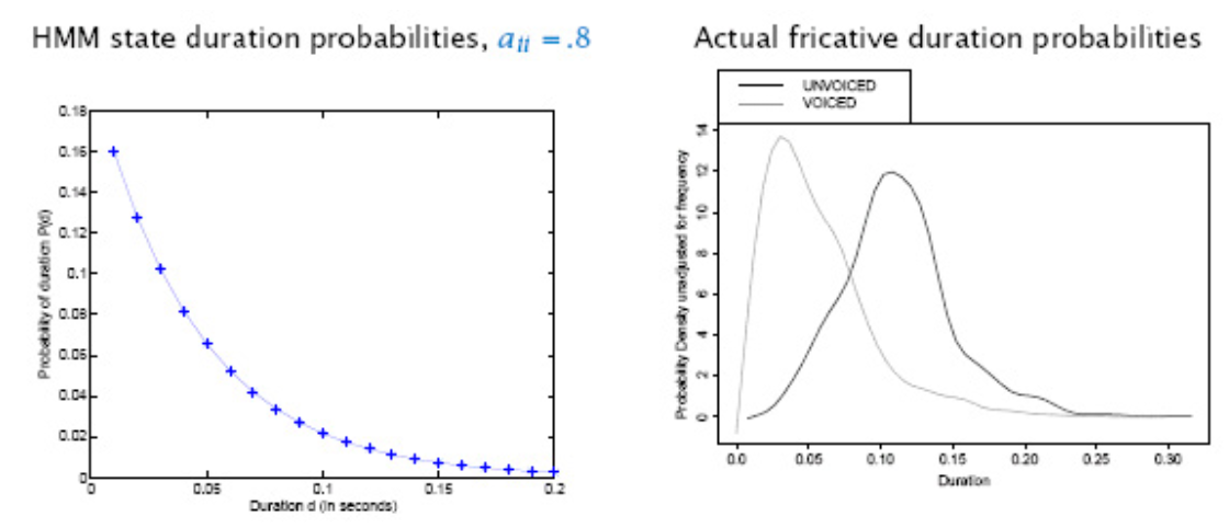
Fig. 140 State Duration Modeling¶

Possible solutions:

Replace transition probabilities with explicit duration distributions [Ostendorf ’96]
- Most general approach
- Breaks dynamic programming algorithms
Replace single state with multiple tied states with identical observation distribution, and some desired transition structure
- Simplest option: Set a minimum duration
- Can simulate other duration distributions with alternative transition structures

Applications¶

HMM can be applied to anything that has “state” and “sequence” attributes.

Automatic speech recognition

One HMM per word or phoneme
Time index corresponds to a 10ms “frame”
Observation is a vector of spectral (frequency) measurements
Can think of HMM state as corresponding to a state of the speaker’s vocal tract

Unsupervised speech unit (Word/Phoneme) Discovery

Learn an HMM to model a collection of unlabelled speech
Group together frequently occurring sequences of states to define units

Activity recognition in video or biometrics

States corresponds to pose
As in speech recognition, the “activity” can be labeled or unlabeled

Speech Tagging

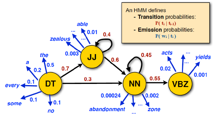
Fig. 141 HMM in part-of-speech tagging [Julia Hockenmeyer]¶

Data Science Handbook