Non-linear Programming
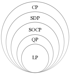
Fig. 12 A hierarchy of convex optimization problems. (LP: linear program, QP: quadratic program, SOCP second-order cone program, SDP: semidefinite program, CP: cone program.) [Wikipedia]
TBC
Primal and Dual short intro.
Lagrange multiplier:
geometric motivation of the method: align tangency of the objective function and the constraints.
formulation of Lagrangean \(\mathcal{L}\): combining all equations to \(\nabla\mathcal{L} = 0\).
interpretation and proof of the Lagrange multiplier \(\lambda\) as \(\frac{\partial f}{\partial c}\), e.g. if budget change, how much will revenue change?
Linear Systems
Consider a system of linear equations: given \(\boldsymbol{A} \in \mathbb{R} ^{m \times n}, \boldsymbol{b} \in \mathbb{R} ^{m}\), we want to find \(\boldsymbol{x} \in \mathbb{R} ^{n}\) such that
Existence and Uniqueness
- Existence
There exists a solution \(\boldsymbol{x}\) to the above equality if and only if
\[ \boldsymbol{b} \in \operatorname{im}(\boldsymbol{A}) \]In this case, we also say that the linear system is consistent.
- Uniqueness
If there exists a solution \(\boldsymbol{x}\), then it is unique if and only if
\[ \operatorname{ker}(\boldsymbol{A}) = \emptyset \]i.e. \(\boldsymbol{A}\) has full column rank.
Otherwise, if \(\boldsymbol{x} _0\) is a solution such that \(\boldsymbol{A} \boldsymbol{x} _0 = \boldsymbol{b}\), then for \(\boldsymbol{x} _1 \ne \boldsymbol{0}, \boldsymbol{x} _1 \in \operatorname{ker}(\boldsymbol{A})\) such that \(\boldsymbol{A} \boldsymbol{x} _1 = \boldsymbol{0}\), we can construct infinite many solutions \(\boldsymbol{x} _0 + c \boldsymbol{x} _1\).
If both conditions are satisfied, there are many ways to solve for \(\boldsymbol{x}\).
Ordinary Least Sqaure
If \(\boldsymbol{b} \notin \operatorname{im}(\boldsymbol{A})\), then we cannot find \(\boldsymbol{x}\) such that \(\boldsymbol{A} \boldsymbol{x} =\boldsymbol{b}\). In this case, we instead find \(\boldsymbol{x}\) such that \(\boldsymbol{A} \boldsymbol{x}\) is the closest to \(\boldsymbol{b}\), where the closeness can be measured by \(L_2\) norm.
This is called a least square method.
The minimizer may not be unique, depending on whether \(\boldsymbol{A}\) has full column rank.
Minimum Length
If the solution (consistent and inconsistent case) is not unique, usually we find the one with minimum length, measured by \(L_2\) norm.
where \(\mathcal{X}\) is the set of solutions to the original problem or least square problem.
To summarize,
consistency \ rank |
\(\boldsymbol{A}\) has full column rank |
Rank deficient |
|---|---|---|
\(\boldsymbol{b} \in \operatorname{im}(\boldsymbol{A})\) |
unique |
minimum length |
\(\boldsymbol{b} \notin \operatorname{im}(\boldsymbol{A})\) |
unique least square |
minimum length leaset square |
First Order Necessary Condition
Consider a minimization problem
For every \(\boldsymbol{x} \in S\), we can define a normal cone,
A necessary condition for optimality of \(\boldsymbol{x} ^*\) for problem \(\min f(\boldsymbol{x})\) is
Imagine that in steepest descent, the trajectory stops at the boundary of \(S\). There is no way to go along the descent direction \(- \nabla f(\boldsymbol{x} ^*)\).
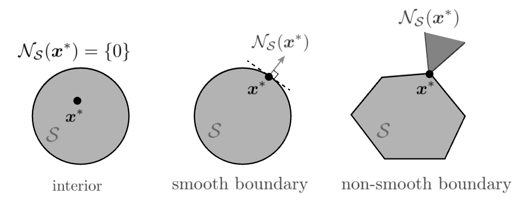
Fig. 13 Normal cones [Friedlander and Joshi]
Rayleigh Quotients
Consider the following constrained optimization where \(\boldsymbol{A}\) is a real symmetric matrix:
An equivalent unconstrained problem is
which makes the objective function invariant to scaling of \(\boldsymbol{x}\). How do we solve this?
- Definition (Quadratic forms)
Let \(\boldsymbol{A}\) be a symmetric real matrix. A quadratic form corresponding to \(\boldsymbol{A}\) is a function \(Q: \mathbb{R} ^n \rightarrow \mathbb{R}\) with
\[ Q_{\boldsymbol{A}}(\boldsymbol{x}) = \boldsymbol{x} ^{\top} \boldsymbol{A} \boldsymbol{x} \]
A quadratic form is can be written as a polynomial with terms all of second order
Basic
- Definition (Rayleigh quotient)
For a fixed symmetric matrix \(\boldsymbol{A}\), the normalized quadratic form \(\frac{\boldsymbol{x} ^{\top} \boldsymbol{A} \boldsymbol{x}}{\boldsymbol{x} ^{\top} \boldsymbol{x} }\) is called a Rayleigh quotient.
In addition, given a positive definite matrix \(\boldsymbol{B}\) of the same size, the quantity \(\frac{\boldsymbol{x} ^{\top} \boldsymbol{A} \boldsymbol{x} }{\boldsymbol{x} ^{\top} \boldsymbol{B} \boldsymbol{x} }\) is called a generalized Rayleigh quotient.
Applications
PCA: \(\max _{\boldsymbol{v} \neq 0} \frac{\boldsymbol{v}^{\top} \boldsymbol{\Sigma} \boldsymbol{v}}{\boldsymbol{v}^{\top} \boldsymbol{v}}\) where \(\boldsymbol{\Sigma}\) is a covariance matrix
LDA: \(\max _{\boldsymbol{v} \neq 0} \frac{\boldsymbol{v}^{\top} \boldsymbol{S}_{b} \boldsymbol{v}}{\boldsymbol{v}^{\top} \boldsymbol{S}_{w} \boldsymbol{v}}\) where \(\boldsymbol{S} _b\) is a between-class scatter matrix, and \(\boldsymbol{S} _w\) is a within-class scatter matrix
Spectral clustering (relaxed Ncut): \(\max _{\boldsymbol{v} \neq \boldsymbol{0}} \frac{\boldsymbol{v}^{\top} \boldsymbol{L} \boldsymbol{v}}{\boldsymbol{v}^{\top} \boldsymbol{D} \boldsymbol{v}} \quad {s.t.} \boldsymbol{v} ^{\top} \boldsymbol{D} \boldsymbol{1} = 0\) where \(\boldsymbol{L}\) is graph Laplacian and \(\boldsymbol{D}\) is degree matrix.
- Theorem (Range of Rayleigh quotients)
For any symmetric matrix \(\boldsymbol{A} \in \mathbb{R} {n \times n}\),
\[\begin{split}\begin{aligned} \max _{\boldsymbol{x} \in \mathbb{R}^{n}: \boldsymbol{x} \neq \boldsymbol{0}} \frac{\boldsymbol{x}^{\top} \boldsymbol{A} \boldsymbol{x}}{\boldsymbol{x}^{\top} \boldsymbol{x}} &=\lambda_{\max } \\ \min _{\boldsymbol{x} \in \mathbb{R}^{n}: \boldsymbol{x} \neq \boldsymbol{0}} \frac{\boldsymbol{x}^{\top} \boldsymbol{A} \boldsymbol{x}}{\boldsymbol{x}^{\top} \boldsymbol{x}} &=\lambda_{\min } \end{aligned}\end{split}\]
That is, the largest and the smallest eigenvalues of \(\boldsymbol{A}\) gives the range for the Rayleigh quotient. The maximum and the minimum is attainted when \(\boldsymbol{x}\) is the corresponding eigenvector.
In addition, if we add an orthogonal constraint that \(\boldsymbol{x}\) is orthogonal to all the \(j\) largest eigenvectors, then
and the maximum is achieved when \(\boldsymbol{x} = \boldsymbol{v} _{j+1}\).
Proof: Linear algebra approach
Consider EVD of \(\boldsymbol{A}\):
where \(\boldsymbol{y} = \boldsymbol{U} ^{\top} \boldsymbol{x}\) is also a unit vector since \(\left\| \boldsymbol{y} \right\| ^2 = 1\). The original optimization problem becomes
Note that the objective and constraint can be written as a weighted sum of eigenvalues
Let \(\lambda_1 \ge \lambda_2 \ge \ldots \ge \lambda_n\), then when \(y_1^2 = 1\) and \(y_2^2 = \ldots = y_n ^2 = 0\), the objective function attains its maximum \(\boldsymbol{y} ^{\top} \boldsymbol{\Lambda} \boldsymbol{y} = \lambda_1\). In terms of \(\boldsymbol{x}\), the maximizer is
In conclusion, when \(\boldsymbol{x} = \pm \boldsymbol{u} _1\), i.e. the largest eigenvector, \(\boldsymbol{x} ^{\top} \boldsymbol{A} \boldsymbol{x}\) attains its maximum value \(\lambda_1\)
Proof: Multivariable calculus approach
Alternatively, we can use the Method of Lagrange Multipliers to prove the theorem. First, we form the Lagrangian function
Differentiation gives
This implies that \(\boldsymbol{x}\) and \(\lambda\) must be an eigenpair of \(\boldsymbol{A}\). Moreover, for any solution \(\lambda=\lambda_{i}, \boldsymbol{x}=\boldsymbol{v}_{i}\), the objective function takes the value
Therefore, the eigenvector \(\boldsymbol{v} _1\) (corresponding to largest eigenvalue \(\lambda_1\) of \(\boldsymbol{A}\)) is the global maximizer, and it yields the absolute maximum value \(\lambda_1\).
Generalized
- Corollary (Generalized Rayleigh quotient problem)
For the generalized Rayleigh quotient \(\frac{\boldsymbol{x}^{\top} \boldsymbol{A} \boldsymbol{x}}{\boldsymbol{x}^{\top} \boldsymbol{B} \boldsymbol{x}}\) where \(\boldsymbol{A}\) is symmetric and \(\boldsymbol{B}\) is p.d., the smallest and largest values \(\lambda\) of the quotient satisfy
The left equation is called a generalized eigenvalue problem.
The smallest/largest quotient value equals the smallest/largest eigenvalue of \((\boldsymbol{B} ^{-1} \boldsymbol{A})\). The number of non-zero eigenvalues is \(r=\operatorname{rank}\left(\boldsymbol{B}^{-1} \boldsymbol{A}\right)\).
The solutions are the corresponding smallest/largest eigenvectors. In some problems, multiple eigenvectors are used, which can be chosen such that
\[\begin{split}\boldsymbol{v} _{i} ^{\top} \boldsymbol{B} \boldsymbol{v}_{j}=\left\{\begin{array}{ll} 1 & \text { if } i=j \leq r \\ 0 & \text { otherwise } \end{array}\right.\end{split}\]
Proof
Substitution approach
Since \(\boldsymbol{B}\) is p.d., we have \(\boldsymbol{B} ^{1/2}\). Let \(\boldsymbol{y} = \boldsymbol{B} ^{1/2}\boldsymbol{x}\), then the denominator can be written as
\[ \boldsymbol{x}^{\top} \boldsymbol{B} \boldsymbol{x}=\boldsymbol{x}^{\top} \boldsymbol{B}^{1 / 2} \boldsymbol{B}^{1 / 2} \boldsymbol{x}=\boldsymbol{y}^{\top} \boldsymbol{y} \]Substitute \(\boldsymbol{x}=\left(\boldsymbol{B}^{1 / 2}\right)^{-1} \boldsymbol{y} \stackrel{\text { denote }}{=} \boldsymbol{B}^{-1 / 2} \boldsymbol{y}\) into the numerator to rewrite it in terms of the new variable \(\boldsymbol{y}\). This will convert the generalized Rayleigh quotient problem back to a regular Rayleigh quotient problem, which has been solved above.
\[ \frac{\boldsymbol{y} \boldsymbol{B} ^{-1/2} \boldsymbol{A} \boldsymbol{B} ^{-1/2} \boldsymbol{y} }{\boldsymbol{y} ^{\top} \boldsymbol{y}} \]The optimum is the eigenvalue \(\lambda\) of \(\boldsymbol{B} ^{-1/2} \boldsymbol{A} \boldsymbol{B} ^{-1/2}\), which is also the eigenvalue of \(\boldsymbol{B} ^{-1} \boldsymbol{A}\) since
\[ \boldsymbol{B} ^{-1/2} \boldsymbol{A} \boldsymbol{B} ^{-1/2}\boldsymbol{v} = \lambda \boldsymbol{v} \quad \Longleftrightarrow \quad \boldsymbol{B} ^{-1} \boldsymbol{A} (\boldsymbol{B} ^{-1/2} \boldsymbol{v} )= \lambda(\boldsymbol{B} ^{-1/2} \boldsymbol{v} ) \]The solution is given by \(\boldsymbol{y} ^* = \boldsymbol{v} ^*\). Then \(\boldsymbol{x} ^* = \boldsymbol{B} ^{-1/2} \boldsymbol{y} ^* = \boldsymbol{B} ^{-1/2} \boldsymbol{v} ^*\), which is the smallest/largest eigenvectors of \(\boldsymbol{B} ^{-1} \boldsymbol{A}\).
Lagrange multipliers approach
\[ \max _{\boldsymbol{x} \neq \boldsymbol{0}}\ \frac{\boldsymbol{x}^{\top} \boldsymbol{A} \boldsymbol{x}}{\boldsymbol{x}^{\top} \boldsymbol{B} \boldsymbol{x}} \]which is equivalent to
\[ \max _{\boldsymbol{x} \in \mathbb{R}^{n}}\ \boldsymbol{x}^{\top} \boldsymbol{A} \boldsymbol{x} \quad \text { subject to } \boldsymbol{x}^{\top} \boldsymbol{B} \boldsymbol{x}=1 \]The Lagrangean is
\[ L(\boldsymbol{x}, \lambda)=\boldsymbol{x}^{\top} \boldsymbol{A} \boldsymbol{x}-\lambda\left(\boldsymbol{x}^{\top} \boldsymbol{B} \boldsymbol{x}-1\right) \]First order conditions:
\[\begin{split} \begin{aligned} \frac{\partial L}{\partial \boldsymbol{x}} &=2 \boldsymbol{A} \boldsymbol{x}-2\lambda \boldsymbol{B} \boldsymbol{x}=0 & \longrightarrow & \boldsymbol{A} \boldsymbol{x}=\lambda \boldsymbol{B}\boldsymbol{x} \\ \frac{\partial L}{\partial \lambda} &=0 & \longrightarrow & \boldsymbol{x} ^{\top} \boldsymbol{B} \boldsymbol{x} =1 \end{aligned} \end{split}\]Hence, the objective is \(\boldsymbol{x} ^{\top} \boldsymbol{A} \boldsymbol{x} = \lambda \boldsymbol{x} ^{\top} \boldsymbol{B} \boldsymbol{x} = \lambda\), where \(\lambda\) satisfies \(\boldsymbol{A} \boldsymbol{x}=\lambda \boldsymbol{B}\boldsymbol{x}\).
In particular, if \(\boldsymbol{A} = \boldsymbol{a} \boldsymbol{a} ^{\top}\) for some \(\boldsymbol{a} \ne \boldsymbol{0}\), the quotient becomes
Obviously, it has minimum \(0\) when \(\boldsymbol{a} ^{\top} \boldsymbol{x} = \boldsymbol{0}\). To find its maximum, we solve the generalized eigen problem
We can see that \(\boldsymbol{v} = c \boldsymbol{B} ^{-1} \boldsymbol{a}\) is an eigenvector with eigenvalue \(\boldsymbol{a} ^{\top} \boldsymbol{B} ^{-1} \boldsymbol{a} > 0\). Since \(\operatorname{rank}\left( \boldsymbol{A} \right) = 1\), it is the only non-zero eigenvalue, i.e. largest eigenvalue.
Another approach is to rearrange and get
Hence \(\boldsymbol{v} = c \boldsymbol{B} ^{-1} \boldsymbol{a}\), \(\lambda = c ^{-1} \boldsymbol{a} ^{\top} \boldsymbol{v}\).
reference:
Semi-definite Programming
We introduce semi-definite programming. Then use it solve max-cut problem, and analyze its performance for min-cut problem over stochastic block model.
Introduction
A linear programming problem is one in which we wish to maximize or minimize a linear objective function of real variables over a polytope. In semidefinite programming, we instead use real-valued vectors and are allowed to take the dot product of vectors. In general, a SDP has a form
The array of real variables in LP is then replaced by an array of vector variables, which form a matrix variable. By using this notation, the problem can be written as
where \(C_{ij} = (c_{ij} + c_{ji})/2, A_{ij}^{(k)} = (a_{ijk} + a_{jik})/2\) and \(\langle \boldsymbol{P}, \boldsymbol{Q} \rangle = \operatorname{tr}\left(\boldsymbol{P} ^{\top} \boldsymbol{Q} \right) = \sum_{i,j}^n p_{ij}q_{ij}\) is the Frobenius inner product.
Note that an \(n \times n\) matrix \(\boldsymbol{M}\) is said to be positive semidefinite if it is the Gramian matrix of some vectors (i.e. if there exist vectors \(\boldsymbol{v} _1, \ldots, \boldsymbol{v} _n\) such that \(M_{ij} = \langle \boldsymbol{v} _i, \boldsymbol{v} _j \rangle\) for all \(i,j\)). Hence, the last constraint is just \(\boldsymbol{X} \succeq \boldsymbol{0}\). That is, the nonnegativity constraints on real variables in LP are replaced by semidefiniteness constraints on matrix variables in SDP.
All linear programs can be expressed as SDPs. SDPs are in fact a special case of cone programming and can be efficiently solved by interior point methods. Given the solution \(\boldsymbol{X}^*\) to the SDP in the standard form, the vectors \(\boldsymbol{v}_1, \ldots, \boldsymbol{v} _n\) can be recovered in \(\mathcal{O} (n^3)\) time, e.g. by using an incomplete Cholesky decomposition of \(\boldsymbol{X}^* = \boldsymbol{V} ^{\top} \boldsymbol{V}\) where \(\boldsymbol{V} = [\boldsymbol{v} _1, \ldots \boldsymbol{v} _n]\).
From Rayleigh Quotient
Recall that an Rayleigh quotient can be formulated as
Since both the objective and the constraint are scalar valued, we can re-write them using trace
Then, by the property of trace, we have
Let \(\boldsymbol{X} = \boldsymbol{x} \boldsymbol{x} ^{\top}\), then the variable \(\boldsymbol{x}\) can be replaced by a rank-1 matrix \(\boldsymbol{X} = \boldsymbol{x} \boldsymbol{x} ^{\top}\)
Note that \(\boldsymbol{X} = \boldsymbol{x} \boldsymbol{x} ^{\top}\) if and only if \(\operatorname{rank}\left( \boldsymbol{X} \right)=1\) and \(\boldsymbol{X} \succeq \boldsymbol{0}\), hence the constraints are equivalent to.
Call this problem RQ, if we drop the rank 1 constraint, then this would be a semidefinite program, where \(\operatorname{tr}\left( \boldsymbol{X} \right)\) can be viewed as \(\langle \boldsymbol{I} , \boldsymbol{X} \rangle = 1\).
In fact, any optimal solution \(\boldsymbol{X} _{SDP}^*\) to this SDP can always be convert to an rank-1 matrix \(\boldsymbol{X} _{RQ}^*\) with the same optimal value. Hence, solving the SDP is equivalent to solving the RQ.
Proof
In SDP, since \(\boldsymbol{X} \succeq \boldsymbol{0}\), let its EVD be \(\boldsymbol{X} = \sum_{i=1}^n \lambda_i \boldsymbol{u}_i \boldsymbol{u}_i ^{\top}\), then the objective function is
Note that \(1 = \operatorname{tr}\left( \boldsymbol{X} \right) = \sum_{i=1}^n \lambda_i\) and \(\lambda_i \ge 0\). Thus, the objective function is a convex combination of \(\operatorname{tr}\left( \boldsymbol{A} \boldsymbol{u} _i \boldsymbol{u} _i ^{\top} \right)\). Hence, for any feasible solution \(\boldsymbol{X} _{SDP} =\sum_{i=1}^n \lambda_i \boldsymbol{u}_i \boldsymbol{u}_i ^{\top}\), we can formulate another rank-1 feasible solution, by selecting \(j = \arg\max_i \operatorname{tr}\left( \boldsymbol{A} \boldsymbol{u} _i \boldsymbol{u} _i ^{\top} \right)\), and setting \(\lambda_j=1\) while \(\lambda_{-j}=0\). The rank-1 feasible solution is then \(\boldsymbol{X} _{RQ} = \boldsymbol{u}_j \boldsymbol{u}_j ^{\top}\), and has a better objective value \(\operatorname{tr}\left( \boldsymbol{A} \boldsymbol{X} _{RQ} \right) \ge \operatorname{tr}\left( \boldsymbol{A} \boldsymbol{X} _{SDP}\right)\). Therefore, for any optimal solution \(\boldsymbol{X} _{SDP}^*\), we can find a rank-1 matrix \(\boldsymbol{X} _{RQ}^*\), such that it is still optimal, since \(\operatorname{tr}(\boldsymbol{A} \boldsymbol{X} _{SDP}^* ) = \operatorname{tr}(\boldsymbol{A} \boldsymbol{X} _{RQ}^* )\).
In this way, the optimal value is then
where the eigenvector \(\left\| \boldsymbol{u} \right\| =1\). This goes back to the formulation of Rayleigh quotient.
For max-cut
In a graph \(G = (V, E)\) with edge weights \(\boldsymbol{W}\), we want to find a maximum bisection cut
where the product \(x_i x_j\) is an indicator variable that equals 1 if two vertices \(i, j\) are in the same part, and \(-1\) otherwise. Hence, the summation only involves the case when \(x_i x_j = -1\), and we divide it by half since \((1- x_i x_j)=2\).
Denote \(\boldsymbol{X} = \boldsymbol{x} \boldsymbol{x} ^{\top} \in \mathbb{R} ^{n \times n}\). Then the domain \(\boldsymbol{x} \in \left\{ \pm 1 \right\}^n\) is bijective to \(\Omega = \left\{ \boldsymbol{X} \in \mathbb{R} ^{n \times n} : \boldsymbol{X} \succeq 0, X_{ii}=1, \operatorname{rank}\left( \boldsymbol{X} \right) = 1 \right\}\). The optimization problem can then be expressed as
Solving this integer optimization is NP-hard. We work with relaxation of \(\Omega\).
Relaxation
We want to relax \(\Omega\) to some continuous domain.
Spectral Relaxation
Two relaxations:
drop the rank 1-constraint \(\operatorname{rank}\left( \boldsymbol{X} \right) = 1\)
replace the diagonal constraint \(X_{ii}=1\) by \(\operatorname{tr}\left( \boldsymbol{X} \right) = n\)
To solve it, it is equivalent to solve
As proved above, this SDP can be solved by solving a Rayleigh quotient problem
The optimal solution \(\boldsymbol{y} ^*\) is the last eigenvector of \(\boldsymbol{W}\), and the objective value is the last eigenvalue of \(\boldsymbol{W}\). The solution to the SDP problem is then \(\boldsymbol{X} ^* = \boldsymbol{y}^* \boldsymbol{y} ^{*\top}\), with the same objective value. We can then round \(\boldsymbol{y} ^*\) by its sign to decide partition assignment.
SDP Relaxation
Only one relaxation: drop the rank-1 constraint, which is non-convex. The remaining two constraints forms a domain
The optimization problem is then
Note that after we drop the rank-1 constraint,
\(\operatorname{SDP}(\boldsymbol{W} ) \ge \operatorname{cut} (\boldsymbol{W})\).
The solution \(\boldsymbol{X} ^*\) to \(\operatorname{SDP} (\boldsymbol{W})\) may not be rank-1. If it is rank-1 then the above equality holds.
It remains to solve \(\operatorname{SDP} (\boldsymbol{W})\) for \(\boldsymbol{X}\), and then find a way to obtain the binary partition assignment \(\hat{\boldsymbol{x}} \in \left\{ \pm 1 \right\}^n\) from \(\boldsymbol{X}\).
Lifting
\(\Omega_{SDP}\) is equivalent to \(\left\{\boldsymbol{X} \in \mathbb{R} ^{n \times n}: \boldsymbol{X} = \boldsymbol{V} ^{\top} \boldsymbol{V}, \left\| \boldsymbol{v} _i \right\| ^2 = 1 \right\}\). In this way, we convert a scalar constraint \(X_{ii}\) to a vector constraint \(\left\| \boldsymbol{v} _i \right\| =1\), aka ‘lifting’.
Random Rounding
Algorithm
Solve \(\operatorname{SDP} (\boldsymbol{W})\) and obtain \(\hat{\boldsymbol{X}}\)
Decompose \(\hat{\boldsymbol{X}} = \hat{\boldsymbol{V}} ^{\top} \boldsymbol{\hat{V}}\), e.g. using EVD \(\boldsymbol{\hat{X}} ^{\top} = \boldsymbol{\hat{U}} \sqrt{\boldsymbol{\hat{\Lambda}}}\), or using Cholesky. Note that \(\left\| \boldsymbol{\hat{v}} _i \right\| =1\) always holds, due to the constraint \(\hat{X}_{ii}=1\).
Sample a direction \(\boldsymbol{r}\) uniformly from \(S^{p-1}\)
Return binary partition assignment \(\hat{\boldsymbol{x}} = \operatorname{sign} (\boldsymbol{\hat{V}} ^{\top} \boldsymbol{r} )\)
Intuition
Randomly sample a hyperplane in \(\mathbb{R} ^n\) characterized by vector \(\boldsymbol{r}\). If \(\hat{\boldsymbol{v}} _i\) lies on the same side of the hyperplane with \(\boldsymbol{r}\), then set \(\hat{x}_i =1\), else \(\hat{x}_i = -1\).
If there indeed exists a partition \(I\) and \(J\) of vertices characterizedd by \(\boldsymbol{x}\), then the two groups of directions \(\boldsymbol{v} _i\)’s and \(\boldsymbol{v} _j\)’s should point to opposite direction since \(\boldsymbol{v} _i ^{\top} \boldsymbol{v} _j = x_i x_j = -1\). After random rounding, they should be well separated. Hence, if \(\hat{\boldsymbol{v}}_i ^{\top} \hat{\boldsymbol{v} }_j\) recovers \(\boldsymbol{v}_i ^{* \top} \boldsymbol{v}^* _j\) well enough, then \(\hat{\boldsymbol{x}}\) well recovers \(\boldsymbol{x}^*\), the optimal max-cut in \(\operatorname{cut}(\boldsymbol{W})\).
To see how \(\boldsymbol{V}\) looks like for \(\boldsymbol{x} \in \left\{ \pm 1 \right\} ^n\), let \(\boldsymbol{x} = [1, 1, -1, -1] ^{\top}\), then
Analysis
How well the algorithm does, in expectation? We define Geomans-Williams quantity, which is the expected cut value returned by the algorithm, where randomness comes from random direction \(\boldsymbol{r}\).
Obviously \(\operatorname{GW} (\boldsymbol{W}) \le \operatorname{cut} (\boldsymbol{W})\), since we are averaging the value of feasible solutions \(\hat{\boldsymbol{x}}\) in \(\left\{ \pm 1\right\}^n\), and each of them is \(\le \operatorname{cut} (\boldsymbol{W})\). But how small can \(\operatorname{GW} (\boldsymbol{W})\) be?
It can be shown that \(\operatorname{GW}(\boldsymbol{W}) \ge \alpha \operatorname{cut}(\boldsymbol{W})\) where \(\alpha \approx 0.87\). That is, the random rounding algorithm return a cut value not too small than the optimal value, in expectation.
Proof
We randomly sample direction \(\boldsymbol{r}\) from unit sphere \(S^{p-1}\). If \(\boldsymbol{v} _i\) and \(\boldsymbol{v} _j\) lie on different side of hyperplane characterized by \(\boldsymbol{r}\), we call such direction ‘good’.
In \(p=2\) case, we sample from a unit circle. All good \(\boldsymbol{r}\) lie on two arcs on the circle, whose length are related to the angle between \(\boldsymbol{v} _i\) and \(\boldsymbol{v} _j\), denoted \(\theta\). The probability of sampling good equals the ratio between the total length of the two arcs and the circumference. Thus,
In \(p = 3\) case, we sample \(\boldsymbol{r}\) from a unit sphere. All good \(\boldsymbol{r}\) lie on two spherical wedges, with angle \(\theta\). The ratio between the area of each spherical wedge and the area of the sphere is \(\theta/2\pi\). An example is given after the proof.
In higher dimensional spaces, we just project \(\boldsymbol{r}\) on to the hyperplane spanned by \(\boldsymbol{v} _i\) and \(\boldsymbol{v} _j\), then it reduces to the \(p=2\) case. Note that the distribution of the projected random \(\boldsymbol{r}\) is still uniform.
Now we compare \(\operatorname{GW}(\boldsymbol{W}) = \sum_{i,j}^n w_{ij} \frac{1}{\pi}\arccos (\boldsymbol{v} _i ^{\top} \boldsymbol{v} _j)\) and \(\operatorname{SDP} (\boldsymbol{W}) = \sum_{i,j}^n w_{ij} \frac{1}{2} (1 - \boldsymbol{v} _i ^{\top} \boldsymbol{v} _j)\).
Let’s first see two functions \(f(y) = \frac{1}{\pi}\arccos(y)\) and \(g(y) = \frac{1}{2}(1-y)\) for \(-1 \le y \le 1\). Let \(\alpha = \min_{-1 \le y \le 1} \frac{f(y)}{g(y)}\), then it is easy to find \(\alpha \approx 0.87\).
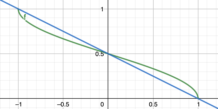
Fig. 14 Plots of \(f(y)\) and \(g(y)\)
Therefore, let \(y_{ij} = \boldsymbol{v} _i \boldsymbol{v} _j\), since \(w_{ij} \ge 0\), we have \(\operatorname{GW} (\boldsymbol{W}) \ge \alpha \operatorname{SDP} (\boldsymbol{W})\). Using the SDP relaxation inequality \(\operatorname{SDP} (\boldsymbol{W}) \ge \operatorname{cut} (\boldsymbol{W})\), we have \(\operatorname{GW} (\boldsymbol{W}) \ge \alpha \operatorname{cut} (\boldsymbol{W})\).
Note that we require \(w_{ij} \ge 0\).
An example of random rounding is given below. Two vectors \(\boldsymbol{v}_1, \boldsymbol{v} _2\) (red, green) and random directions \(\boldsymbol{r}\) (blue) from unit sphere whose corresponding hyperplane separates the two vectors.
import numpy as np
import plotly.express as px
import plotly.io as pio

v = np.array([[1,0,3], [-1,0,3]]) # v1, v2
v = v/np.linalg.norm(v, 2, axis=1)[:, np.newaxis]
n = 3000
np.random.seed(1)
x = np.random.normal(size=(n,3))
x = x / np.linalg.norm(x, 2, axis=1)[:, np.newaxis]
x = x[np.dot(x,v[0])*np.dot(x,v[1]) <0, :]
print(f'v1 = {np.round(v[0],3)}, \nv2 = {np.round(v[1],3)}')
print(f'arccos(v1,v2)/pi = {np.round(np.arccos(v[0] @ v[1].T)/np.pi,3)}')
print(f'simulated result = {np.round(len(x)/n,3)}')

pio.renderers.default = "notebook" # renderer
fig = px.scatter_3d(x=x[:,0], y=x[:,1], z=x[:,2], size=np.ones(len(x)), range_z=[-1,1])
fig.add_scatter3d(x=[0, v[0,0]], y=[0, v[0,1]], z=[0, v[0,2]], name='v1')
fig.add_scatter3d(x=[0, v[1,0]], y=[0, v[1,1]], z=[0, v[1,2]], name='v2')
fig.show()
v1 = [0.316 0.    0.949],
v2 = [-0.316  0.     0.949]
arccos(v1,v2)/pi = 0.205
simulated result = 0.208
Besides, how large can the SDP relaxation value \(\operatorname{SDP} (\boldsymbol{W})\) be? Grothendieck’s Inequality says
where \(K \approx 1.7\). Hence, the SDP relaxation \(\Omega_{SDP}\) does not relax the original domain \(\Omega\) too much (otherwise we may see \(\operatorname{SDP}(\boldsymbol{W}) \gg \operatorname{cut}(\boldsymbol{W})\)). Hence \(\hat{\boldsymbol{v}}_i ^{\top} \boldsymbol{\hat{v}} _j\) should recover binary \(x_i^* x_j^*\) well.
To analyze it more specifically, we impose some structural assumption of \(\boldsymbol{W}\), e.g. that from SBM.
For min-cut
The above inequalities applies to any problem instance \(G=(V, E, \boldsymbol{W})\). It may give too generous or useless guarantee for some particular model. Let’s see its performance in stochastic block models.
Formulation
Let \(\boldsymbol{A}\) be a random SBM adjacency matrix. Recall that
We work with another matrix \(\boldsymbol{B} = \left( \boldsymbol{A} - \frac{p+q}{2} \boldsymbol{1} \boldsymbol{1} ^{\top} \right)\). In expectation,
which is a rank-1 matrix. With noise \(\boldsymbol{E}\), we observe \(\boldsymbol{B} = \mathbb{E} [\boldsymbol{B}] + \boldsymbol{E}\), which is no longer rank-1. In this case, we approximate the unknown \(\mathbb{E} [\boldsymbol{B}]\) with a rank-1 matrix \(\boldsymbol{X} = \boldsymbol{x} \boldsymbol{x} ^{\top}\), by maximizing \(\langle \boldsymbol{B}, \boldsymbol{X} \rangle\).
We hope that the optimal solution looks like
which recovers the cluster label. Similar to the max-cut case, we apply SDP relaxation that drops the non-convex rank-1 constraint to \(\boldsymbol{X}\). The SDP problem is then
Note \(\operatorname{tr}\left( \boldsymbol{B} \boldsymbol{X} \right) = \langle \boldsymbol{B} , \boldsymbol{X} \rangle = \sum_{i,j}^n b_{ij} x_{ij}\). Next, we show that the solution to the relaxed problem, denoted \(\hat{\boldsymbol{X}}\), is exactly \(\boldsymbol{X} ^*\). Hence, even though we’ve dropped the rank-1 constraint, we can still solve the relaxed problem and exactly recover the cluster labels.
Dual Problem
First we convert it to an equivalent minimization problem
The Lagrangean is
where \(\boldsymbol{z} \in \mathbb{R} ^n\) and \(\boldsymbol{\Lambda} \succeq \boldsymbol{0}\) are dual variables. Then the constraint primal minimization problem is equivalent to the unconstraint min-max problem on the LHS below.
The above inequality is from minimax inequality (Sion’s minimax theorem). In LP, the equality always holds. In SDP, under some mild condition (Slater’s condition) it holds. Now we solve the RHS dual problem. For the inner minimization problem \(\min_{\boldsymbol{X}} \mathcal{L} (\boldsymbol{X} ; \boldsymbol{z} , \boldsymbol{\Lambda})\), take partial derivative w.r.t. \(\boldsymbol{X}\).
where \(\operatorname{diag}(\boldsymbol{z})\) is an \(n\times n\) diagonal matrix. Plug this identity back to \(\mathcal{L}\) gives the RHS outer maximization problem
There are conditions for optimality of primal and dual variables \((\boldsymbol{X} , \boldsymbol{z} , \boldsymbol{\Lambda})\), called KKT condition:
primal feasible: \(\boldsymbol{X} \succeq \boldsymbol{0}, X_{ii}=1\)
dual feasible: \(\boldsymbol{\Lambda} \succeq \boldsymbol{0} , - \boldsymbol{B} - \operatorname{diag}\left( \boldsymbol{z} \right) - \boldsymbol{\Lambda} = \boldsymbol{0}\)
complementary slackness: \(\langle \boldsymbol{\Lambda} , \boldsymbol{X} \rangle = 0 \Leftrightarrow \boldsymbol{\Lambda} \boldsymbol{X} = \boldsymbol{0}\)
Next we show
Given \(\boldsymbol{B} = \mathbb{E} [\boldsymbol{B}] + \boldsymbol{E}\), there exists \(\boldsymbol{z}, \boldsymbol{\Lambda}\) such that \((\boldsymbol{X} ^*, \boldsymbol{z} , \boldsymbol{\Lambda})\) satisfies KKT condition. Hence \(\boldsymbol{X} ^*\) is an optimal solution to the relaxed problem.
This triple also satisfies one additional condition \(\operatorname{rank}\left( \boldsymbol{\Lambda} \right) + \operatorname{rank}\left( \boldsymbol{X} ^* \right) = n\), called strict complementary condition.
If KKT conditions and this strict complementary condition hold, \(\boldsymbol{X} ^*\) is the unique optimizer.
Note that in the above setting
such \(\boldsymbol{z} , \boldsymbol{\Lambda}\) aka dual certificate
complementary slackness \(\boldsymbol{\Lambda} \boldsymbol{X} = \boldsymbol{0}\) says has some null space, i.e. \(\operatorname{dim} (\operatorname{null} (\boldsymbol{\Lambda})) \ge 1\), but the strict complementary condition says it is exactly \(1\).
Geometric meaning of dual certificate: normal cone
We briefly introduce the normal cone for this problem, which helps to understand the KKT conditions on dual certificate. For the simpler case where variable is a vector \(\boldsymbol{x} \in \mathbb{R} ^n\), see here.
Recall the original problem can is
The feasible region can be specified as
where \(\boldsymbol{C} _i = \boldsymbol{e} _i \boldsymbol{e} _i ^{\top}, b_i = 1\). The normal cone of \(\boldsymbol{S}\) at \(\boldsymbol{x}\) is
Note that \(- \nabla f(\boldsymbol{X}) = \boldsymbol{B}\). By the first order necessary condition \(- \nabla f(\boldsymbol{X}) \in N_S(\boldsymbol{X})\), we have
\(\boldsymbol{B} = \sum_{i=1}^n \lambda_i \boldsymbol{C} _i - \boldsymbol{\Lambda}\) for some \(\lambda_i\). By viewing \(z_i = -\lambda_i \in \mathbb{R}\), this equation is exactly the zero partial derivative of Lagrangean \(\frac{\partial \mathcal{L} }{\partial \boldsymbol{X}} = -\boldsymbol{B} - \operatorname{diag}\left( \boldsymbol{z} \right) - \boldsymbol{\Lambda} = 0\)
\(\boldsymbol{\Lambda} \succeq \boldsymbol{0}, \langle \boldsymbol{\Lambda} , \boldsymbol{X} \rangle = 0\), which are dual feasibility and complementary slackness.
Uniqueness
KKT implies optimality of \(\boldsymbol{X}^*\). To show why the additional strict complementary condition implies uniqueness, let \(\boldsymbol{X} = \boldsymbol{X} ^* + \Delta\) be another optimizer. Then
Proof idea
The idea is to decompose \(\Delta = \boldsymbol{X} - \boldsymbol{X}^*\) into two orthogonal components, parallel component \(P_{\boldsymbol{X} ^{*\parallel}} (\Delta)\) to \(\boldsymbol{X} ^*\) and orthogonal component \(P_{\boldsymbol{X} ^{* \perp}} (\Delta)\) to \(\boldsymbol{X} ^*\). Then show \(P_{\boldsymbol{X}^ {* \perp}} (\Delta)\) is zero. Hence only the parallel component remains, i.e. \(\boldsymbol{X}\) is some ‘scaling’ of \(\boldsymbol{X}^*\).
Let \(\boldsymbol{u} = \frac{1}{\sqrt{n}} \left[\begin{array}{cc} \boldsymbol{1} \\ -\boldsymbol{1} \end{array}\right]\) to be normalized \(\boldsymbol{x} ^*\), and let \(\boldsymbol{U} \in \mathbb{R} ^{n \times (n-1)}\) be orthonormal basis of subspace of \(\mathbb{R} ^n\) that is orthogonal to \(\boldsymbol{u}\). By KKT.3 \(\boldsymbol{\Lambda} \boldsymbol{X} ^* = \boldsymbol{0}\), then \(\boldsymbol{\Lambda} \boldsymbol{u} =0\), i.e. \(\boldsymbol{u} \in \operatorname{null} (\boldsymbol{\Lambda})\), we can write \(\boldsymbol{\Lambda} = \boldsymbol{U} \tilde{\boldsymbol{\Lambda} } \boldsymbol{U} ^{\top}\) where \(\tilde{\boldsymbol{\Lambda}} \in \mathbb{S}_+ ^{n-1}\). Substituting this back to the above equation gives
Note two facts
Recall that \(\boldsymbol{X} = \boldsymbol{X} ^* + \Delta\), we have
\[\begin{split}\begin{aligned} \boldsymbol{U} ^{\top} \Delta \boldsymbol{U} &=\boldsymbol{U} ^{\top} (\boldsymbol{X} - \boldsymbol{X} ^*) \boldsymbol{U} \\ &= \boldsymbol{U} ^{\top} \boldsymbol{X} \boldsymbol{U} \quad \because \boldsymbol{U} ^{\top} \boldsymbol{u} = \boldsymbol{0}_{n-1}\\ &\succeq \boldsymbol{0}_{(n-1) \times n-1} \quad \because \boldsymbol{X} \succeq \boldsymbol{0}_{n \times n} \end{aligned}\end{split}\]This observation states the difference \(\Delta\) in orthogonal space spanned by \(\boldsymbol{U}\) is p.s.d.
By strict complementary condition, we have \(\lambda_{\min}(\tilde{\boldsymbol{\Lambda}}) > 0\), otherwise \(\boldsymbol{\Lambda}\) is rank-2 deficient, contradict to \(\operatorname{rank}(\boldsymbol{\Lambda}) = n-1\).
By these two facts, we have
Since \(X_{ii} = 1\), we have \(a=n\), i.e. \(\boldsymbol{X} = \boldsymbol{X} ^*\).
Solve Dual Variables
To find \(\boldsymbol{\Lambda}, \boldsymbol{z}\), by KKT.3, \(\boldsymbol{\Lambda} \boldsymbol{x} ^* = \boldsymbol{0}\), hence
Then we solve for \(\boldsymbol{z}\)
where \(\mathbb{I}= -1\) if \(1\le i \le \frac{n}{2}\) and \(1\) otherwise. Note that the two clusters have the same size \(n/2\). We then substitute this to find \(\boldsymbol{\Lambda}\).
By construction, \(\boldsymbol{z} , \boldsymbol{\Lambda}\) satisfies KKT.3 complementary slackness and 1st order necessary condition. We also need to show \(\boldsymbol{\Lambda} \succeq \boldsymbol{0}\) and the strict complementary condition \(\operatorname{rank}(\boldsymbol{\Lambda} ) = n -1\).
Let \(\boldsymbol{J} = \boldsymbol{I} - \frac{1}{n} \boldsymbol{x}^* \boldsymbol{x}^{* \top}\). Then \(\boldsymbol{J}\) is a projection matrix to orthogonal space of \(\boldsymbol{x}^*\).
If \((- \operatorname{diag}(\boldsymbol{z}) - \boldsymbol{E})\) is p.d, then \(\boldsymbol{\Lambda} \succeq \boldsymbol{0}\) and \(\operatorname{rank}(\boldsymbol{\Lambda} ) = n -1\). Now we show it indeed holds. Since \(\boldsymbol{E}\) is symmetric, it is equivalent to show that
Recall definitions and facts
\(A_{ij} \sim \operatorname{Ber}(p)\) or \(\operatorname{Ber}(q)\).
\(\boldsymbol{E} = \boldsymbol{A} - \mathbb{E} [\boldsymbol{A} ] = \boldsymbol{B} - \mathbb{E} [\boldsymbol{B}]\).
\(\mathbb{E} [\boldsymbol{B}] = \frac{p-q}{2} \left[\begin{array}{c} \boldsymbol{1} \\ -\boldsymbol{1} \end{array}\right] \left[\begin{array}{cc} \boldsymbol{1} ^{\top} & - \boldsymbol{1} ^{\top} \\ \end{array}\right]\)
\(\left\| \boldsymbol{E} \right\|_2 = \mathcal{O} (\sqrt{n p \log n})\) for \(p > q \ge \frac{b \log n}{n}\)
\(\sigma_\max (\boldsymbol{E} ) \ge \lambda_\max (\boldsymbol{E} )\) since \(\boldsymbol{E}\) is symmetric
\(\sum_j E_{ij} = \mathcal{O} (\sqrt{n p \log n})\) w.h.p. by Hoeffding’s inequality
Substituting (2) into the above equation for \(\boldsymbol{z}\) gives
In scalar form,
By fact (4) and (5), to ensure \(- z_i \ge \lambda_\max (\boldsymbol{E} )\), a necessary condition is
To ensure this, substituting the scalar form of \(-z_i\), a necessary condition is
Therefore, as long as this holds, then \((- \operatorname{diag}(\boldsymbol{z}) - \boldsymbol{E})\) is p.d, and hence we have exactly recovery of \(\boldsymbol{x}^*\).
Algorithms for SDP
interior point: slow, but arbitrary accuracy
augmented Lagrangian method: faster, but limited accuracy
ADMM
Compressed sensing
Aka sparse sampling.
Note on convex relaxation
Suppose we have some low-dimensional object in high-dimensional space. Our goal is to retrieve these low-dimensional object via some sparse measurement. The key is that the sensing mechanism is ‘incoherent’ with the object.
Problem
We want to find solution \(\boldsymbol{x}\) to the linear system
\(\boldsymbol{A} \in \mathbb{R} ^{n \times p}, \boldsymbol{b} \in \mathbb{R} ^n\)
\(\boldsymbol{x} \in \mathbb{R} ^{p}\)
\(n < p\), less equations than unknowns
Since \(n < p\), there is no unique solution.
Relaxation
We need impose some structure on \(\boldsymbol{x}\) to ensure uniqueness. For instance, a sparse structure: \(\boldsymbol{x}\) have only \(k\) non-zero entries. If we know the support \(S = \operatorname{supp} (\boldsymbol{x})\), i.e. where the non-zero entries are, then ideally a necessary condition for uniqueness is \(n \ge k\). We just need to solve \(\boldsymbol{A} _S \boldsymbol{x} _S = \boldsymbol{b}\).
One can thus solve
where \(\left\| \boldsymbol{x} \right\| _0\) is the cardinality of \(\boldsymbol{x}\). We penalize it.
However, this subset-selection problem is NP-hard. The \(\left\| \cdot \right\| _0\) is non-smooth, non-convex. Can we find \(\left\| \cdot \right\| _\alpha\) from \(\alpha\) where \(\alpha > 0\) such that it approximates \(\left\| \cdot \right\| _0\)? For instance, \(\left\| \cdot \right\| _{1/2}\) is also non-smooth, non-convex. The nearest possible convex relaxation is \(\left\| \cdot \right\| _1\).
The problem becomes
which aka basis pursuit (BP). We hope this is tractable.
Recovery
How good the solution to \(\text{P}_1\) recovers sparse ground truth \(\boldsymbol{x} ^*\) to \(\text{P}_0\)?.
Geometrically, the iso-surface of \(\left\| \boldsymbol{x} \right\|_1\) is pointy. It is very likely that the solution lies in some axis, i.e. sparse solution.
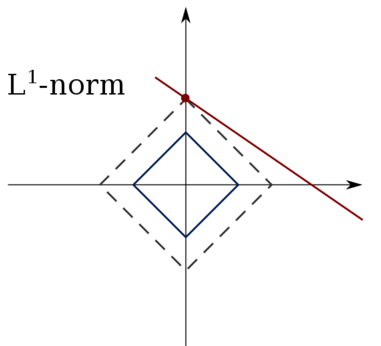
Fig. 15 The constraint \(\boldsymbol{a} ^{\top} \boldsymbol{x} =b\) is a line, since \(1=n < p=2\). The solution is very likely to lie on an axis.
Note that basis pursuit cannot recover \(\boldsymbol{x} ^*\) for all \(\boldsymbol{A}\) (otherwise ‘P=NP’). It recovers \(\boldsymbol{x} ^*\) for some \(\boldsymbol{A}\), that satisfies one of the following conditions/properties. Either is sufficient.
irrepresentable condition
restricted isometry property (RIP)
We now illustrate these two conditions with details. Recall that
\(S = \operatorname{supp} (\boldsymbol{x})\)
\(\boldsymbol{A} = [\boldsymbol{A} _S\quad \boldsymbol{A} _{S^c}]\)
\(\boldsymbol{x} = \left[\begin{array}{c} \boldsymbol{x} _S \\ \boldsymbol{x} _{S^c} \end{array}\right]\)
\(\boldsymbol{x}^* = \left[\begin{array}{c} \boldsymbol{x} _S ^* \\ \boldsymbol{0} \end{array}\right]\)
Irrepresentable Condition
\(\left\| (\boldsymbol{A} _S ^{\top} \boldsymbol{A} _S) ^{-1} \boldsymbol{A} _S ^{\top} \boldsymbol{A} _{S^c} \right\|_\infty < 1\)
An eigenvalue lower bound \(\lambda_\min (\boldsymbol{A} ^{\top} _S \boldsymbol{A} _S ) \ge r\), or equivalently \(\boldsymbol{A} ^{\top} _S \boldsymbol{A} _S \ge r \boldsymbol{I} _k\). Otherwise, solving \(\boldsymbol{A} _S \boldsymbol{x} _S = \boldsymbol{b}\) involves a high condition number matrix.
For \(\boldsymbol{x} ^*\) such that \(\boldsymbol{A} \boldsymbol{x} ^* = \boldsymbol{b}\), then \(\boldsymbol{A} ^{\top} \boldsymbol{A} \boldsymbol{x} ^* = \boldsymbol{A} ^{\top} \boldsymbol{b}\), written in block matrix form
If \(\hat{\boldsymbol{x} } \ne \boldsymbol{x} ^*\) s.t. \(\hat{S}= \operatorname{supp}(\hat{\boldsymbol{x}}), \boldsymbol{b} = \boldsymbol{A} \hat{\boldsymbol{x} }\), we want to show \(\left\| \hat{\boldsymbol{x}} \right\| _1 > \left\| \boldsymbol{x} ^* \right\| _1\), hence \(\boldsymbol{x} ^*\) is the unique solution to \(\text{P}_1\).
The second last inequality holds since
Restricted Isometry Property
- Definition (Restricted Isometry Property)
Let \(\boldsymbol{A}\) be an \(n \times p\) matrix and let \(1 \le k \le p\) be an integer. Suppose there exists a constant \(\delta_k \in (0,1)\) s.t.
for every \(n \times k\) submatrix \(\boldsymbol{A} _k\) of \(\boldsymbol{A}\)
for every \(k\)-dimensional vector \(\boldsymbol{x} \)
\[ (1 - \delta_k) \left\| \boldsymbol{x} \right\| _2 ^2 \le \left\| \boldsymbol{A}_k \boldsymbol{x} \right\| _2 ^2 \le (1 + \delta_k) \left\| \boldsymbol{x} \right\| _2 ^2 \]Then \(\boldsymbol{A}\) is said to satisfy the \(k\)-restricted isometry property with restricted isometry constant \(\delta_k\).
This is equivalent to stating that
\(\left\| \boldsymbol{A} ^{\top} _k \boldsymbol{A} _k - \boldsymbol{I} \right\|_2 \le \delta_{k}\), or
all eigenvalues of \(\boldsymbol{A} ^{\top} _k \boldsymbol{A} _k\) are in the interval \([1 - \delta_k, 1+ \delta_k]\)
The RIC constant is defined as the infimum of all possible \(\delta\) for a given \(\boldsymbol{A}\).
The restricted isometry property characterizes matrices which are nearly orthonormal.
- Theorem (Candes-Tao 2006)
For \(\boldsymbol{x} ^*\) that is \(k\)-sparse and \(\boldsymbol{A} \boldsymbol{x} ^* = \boldsymbol{b}\), if \(\boldsymbol{A}\) satisfies \(2k\)-restricted isometry property with RIC coefficient \(\delta_{2k} < \sqrt{2}-1\), then basis pursuit method recovers \(\boldsymbol{x} ^*\).
Implication: if \(n\) is too small, then \(\delta\) is small (from JL Lemma), such that the inequality cannot hold. Hence, this theorem gives a lower bound of \(n\), which is \(n \ge k \log \frac{p}{k}\). This says that to recover \(k\)-sparse \(\boldsymbol{x} ^*\), we do not need too many equations. Just slightly larger than \(k\) (by a factor of \(\log \frac{p}{k}\)) is enough.
Comment on Sensing
Problem
How to sense/recover a high-dimensional object with smaller number of measurements? For instance,
In SDP for SBM min-cut, the underlying signal is \(n \times n\) matrix \(\boldsymbol{X} = \boldsymbol{x} \boldsymbol{x} ^{\top}\). Since \(p \sim q \sim \mathcal{O} (\frac{\log n}{n} )\), the number of non-zero entries in the \(n \times n\) adjacency matrix \(\boldsymbol{A}\) is \(\mathcal{O} (n \log n)\). We want to recover \(n \times n\) object \(\boldsymbol{X}\) from \(\mathcal{O} (n \log n)\) measurements in \(\boldsymbol{A}\).
In compressed sensing, the underlying signal is \(\boldsymbol{x} \in \mathbb{R} ^{p}\), we have \(\boldsymbol{A} \in \mathbb{R} ^{n \times p}\) where \(n \le p\). We want to recover \(p\)-dim object \(\boldsymbol{x}\) from \(n \le p\) measurements.
Condition for Recovery
Two conditions for good recovery
there exists certain structure of underlying object, e.g.
the matrix is low-rank \(\boldsymbol{X} = \boldsymbol{x} \boldsymbol{x} ^{\top}\),
the vector \(\boldsymbol{x} \in \mathbb{R} ^{p}\) is sparse.
measurements are incoherence with the underlying object
Incoherence
Let \(S\) be a set of measurements \(\boldsymbol{M}\). Usually \(S\) forms an orthonormal basis, i.e.
if \(\boldsymbol{M} \in \mathbb{R} ^{n}\) then \(\boldsymbol{M}_i = \boldsymbol{e} _i\).
if \(\boldsymbol{M} \in \mathbb{R} ^{n \times n}\) then \(\boldsymbol{M}_{ij} = \boldsymbol{e} _i \boldsymbol{e} _j ^{\top}\).
Coherence vs Incoherence
If \(\langle \boldsymbol{M} , \boldsymbol{X} \rangle\) is large for some specific measurements \(\boldsymbol{M} \in S\) and very small for others, then we say measurement set \(S\) is coherent with \(\boldsymbol{X}\). For instance, \(\boldsymbol{M}_i = \boldsymbol{e} _i, \boldsymbol{X} = [1, 0, \ldots, 0]\). In this case, it is hard to find the good \(\boldsymbol{M}\) that has large \(\langle \boldsymbol{M} , \boldsymbol{X} \rangle\) value. We need many number of measurements.
If \(\langle \boldsymbol{M} , \boldsymbol{X} \rangle\) is small for all \(\boldsymbol{M} \in S\), then we say measurement set \(S\) is incoherent with \(\boldsymbol{X}\). For instance, \(\boldsymbol{M}_i = \boldsymbol{e} _i, \boldsymbol{X} = \boldsymbol{1}/\sqrt{n}\). Though each \(\langle \boldsymbol{M}_i , \boldsymbol{X} \rangle\) is small, but each contributes some quantity to the overall.
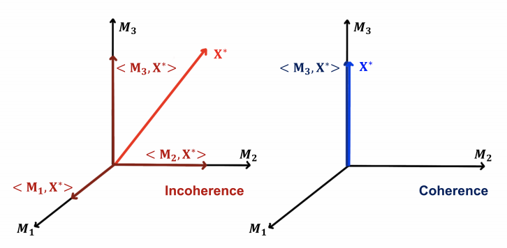
Fig. 16 Incoherence vs coherence [Hieromnimon, Xu, and Fu 2021]
Example of incoherence: SDP for SBM min-cut
Recall that in SDP for SBM min-cut we want to maximize
We can re-write this inner product as
Let \(\boldsymbol{M} _{ij} = a_{ij} \boldsymbol{e} _i \boldsymbol{e} _j ^{\top} - \frac{p+q}{2}\), then
In other words, although small, every single \((i,j)\) observation contributes something information about \(\boldsymbol{X}\).
Example of incoherence: randomized SVD
Incoherence is the reason why we pick random Gaussian directions for randomized SVD. Recall that, for Gaussian random vector \(\boldsymbol{m} \sim \mathcal{N} _p (\boldsymbol{0} , p ^{-1} \boldsymbol{I} )\) and some constant vector \(\boldsymbol{a} \in \mathbb{R} ^{p}\), we have
Although small, every single random measurement \(\boldsymbol{m}\) contributes something information about \(\boldsymbol{a}\).