Common Tests
Theories
We first introduce some theories for statistical inference.
Sample Statistics
For a random sample \((X_1, \ldots, X_n)\), the sample mean and sample variance can be computed as
They are unbiased estimators since
where we used the fact that \(\mathbb{E} [\bar{X}^2] = \operatorname{Var}\left( \bar{X} \right) + \mathbb{E} [\bar{X}] ^2 = \frac{1}{n} \sigma^2 + \mu^2\).
If the random variables are i.i.d. sampled from normal distribution \(X_i \overset{\text{iid}}{\sim} \mathcal{N}\), then \(\bar{X}\) and \(S^2\) (both are random) are independent.
Distribution Derived from Normal
Standard Normal Distributions
If \(X_i \overset{\text{iid}}{\sim} \mathcal{N} (\mu, \sigma^2)\), then
Proof
Since \(X_i \overset{\text{iid}}{\sim}\mathcal{N} (\mu, \sigma)\), then \(Z_i = \frac{ X_i - \mu}{ \sigma} \overset{\text{iid}}{\sim} \mathcal{N} (0, 1)\)
Chi-squared Distributions
If \(Z_i \overset{\text{iid}}{\sim} \mathcal{N} (0, 1)\), then their squared sum follows Chi-squared distribution with degree of freedom \(n\), mean \(n\), and variance \(2n\).
If \(X_i \overset{\text{iid}}{\sim} \mathcal{N} (\mu, \sigma^2)\), then we can find a distribution for the sample variance \(S^2\) as
which does not depends on the true mean \(\mu\).
\(t\) Distributions
If \(Z \sim \mathcal{N} (0, 1)\), and \(V \sim \chi ^2 _n\) and \(Z\) and \(V\) are independent, then
In short, an independent standard normal random variable and a chi-squared random variable can be used to construct a \(t\) distribution. We will use this lemma in a moment.
If \(X_i \overset{\text{iid}}{\sim} \mathcal{N} (\mu, \sigma^2)\), then
Proof
Rewritting the LHS gives
For the numerator we have shown that \(Y=\sqrt{n} \frac{\bar{X} - \mu}{\sigma} \sim \mathcal{N} (0, 1)\). For the ratio in the denominator \(V = \frac{(n-1)S^2}{\sigma^2} \sim \chi ^2 _{n-1}\) by the theorem above. Also note that \(Y\) and \(V\) are independent since \(\bar{X}\) and \(S^2\) are independent. By the theorem above, the \(\frac{Y}{\sqrt{V/(n-1)}}\) follows a \(t\) distribution with d.f. \(n-1\).
Confidence Intervals
Given a sample \((X_1, \ldots, X_n)\), we want to find two bounds \(\hat{\theta}_L\) and \(\hat{\theta}_R\) for the unknown parameter \(\theta\), such that \(\mathbb{P} (\hat{\theta}_L <\theta < \hat{\theta}_R) = 1- \alpha\). The interval \((\hat{\theta}_L, \hat{\theta}_R)\) is called the \((1-\alpha)\%\) confidence interval.
We first give a summary table and then introduce the details.
Scenario |
Distribution |
C.I |
|---|---|---|
Normal Means (known \(\sigma\)) |
\(\frac{\bar{X} - \mu}{\sigma/\sqrt{n}} \sim \mathcal{N} (0, 1)\) |
\(\bar{X} \pm z_{\alpha/2} \frac{\sigma}{\sqrt{n}}\) |
Normal Means (unknown \(\sigma\)) |
\(\frac{\bar{X} - \mu}{S/\sqrt{n}} \sim t_{n-1}\) |
\(\bar{X} \pm t_{\alpha/2} \frac{S}{\sqrt{n}}\) |
Normal Variance |
\(\frac{(n-1)S^2}{\sigma^2 } \sim \chi ^2 _{n-1}\) |
\(\left(\frac{(n-1) S^{2}}{\chi_{R, n-1}^{2}}, \frac{(n-1) S^{2}}{\chi_{L, n-1}^{2}}\right)\) |
General Means (\(n \ge 30\)) |
\(\frac{\left(\bar{X}-\mu\right)}{\sigma/\sqrt{n}}\overset{\mathcal{D}}{\rightarrow} \mathcal{N}(0,1)\) |
\(\bar{X} \pm z_{\alpha/2} \frac{\sigma}{\sqrt{n}}\) (*) |
\(*\) Approximate. Replace \(\sigma\) by \(S\) if \(\sigma\) is unknown.
CI for Normal Means
Known Variance
Suppose the observations are from a normal distribution, \(X_i \overset{\text{iid}}{\sim} \mathcal{N} (\mu, \sigma^2)\) where \(\sigma^2\) is known. We have shown that
Hence, from the standard normal distribution, we can find the cutoff \(z_{\alpha/2}\) such that
Substituting \(Z = \frac{\bar{X} - \mu}{\sigma/\sqrt{n}}\) gives the confidence interval for \(\mu\).
Sometimes people just write \(\bar{X} \pm z_{\alpha/2} \frac{\sigma}{\sqrt{n}}\).
Unknwon Variance
Suppose the observations are from a normal distribution, \(X_i \overset{\text{iid}}{\sim} \mathcal{N} (\mu, \sigma^2)\) where \(\sigma^2\) is unknown. We have shown that
Hence, from the \(t_{n-1}\) distribution, we can find a cutoff \(t_{\alpha/2}\) such that
Substituting \(T = \frac{\bar{X} - \mu}{S/\sqrt{n}}\) gives the confidence interval for \(\mu\).
Sometimes people just write \(\bar{X} \pm t_{\alpha/2} \frac{S}{\sqrt{n}}\).
Why “Confidence”?
Note that the confidence interval \(\left( \bar{X} - t_{\alpha/2} \frac{S}{\sqrt{n}}, \bar{X} + t_{\alpha/2} \frac{S}{\sqrt{n}} \right)\) is a random interval; its center \(\bar{X}\) and its width \(t_{\alpha/2} \frac{S}{\sqrt{n}}\) both depend on the data. After generating the data and calculating \(\bar{X}\) and \(S^2\), this gives us a specific interval. It is no longer accurate to say that \(\mathbb{P} (\mu \in \text{interval} ) = 1-\alpha\); the statement is either TRUE or FALSE (i.e. the event \(\left\{ \mu \in \text{interval} \right\}\) has already either occurred or not).
However, we cannot see whether it’s true or false as we don’t know \(\mu\). Since before drawing the data we had a \(1-\alpha\) probability of construting an interval for which the statement is true, we now say that we have \(1-\alpha\) confidence that the statement is true. This is a confidence interval for \(\mu\).
CI for Normal Variances
Suppose the observations are from a normal distribution, \(X_i \overset{\text{iid}}{\sim} \mathcal{N} (\mu, \sigma^2)\) where \(\sigma^2\) is unknown. We have shown that
Let \(\chi ^2 _{L, n-1}\) and \(\chi ^2 _{R, n-1}\) be positive number such that
Then replacing \(W\) by \(\frac{(n-1)S^2}{\sigma^2 }\) in the above we obtain
Therefore
is a \(1-\alpha\) confidence interval for \(\sigma^2\).
Note that the \(\chi ^2\) distribution is not symmetric. A common way to choose \(\chi ^2 _{L, n-1}\) and \(\chi ^2 _{R, n-1}\) is such that the two tail probabilities are both \(\alpha/2\), as shown below.
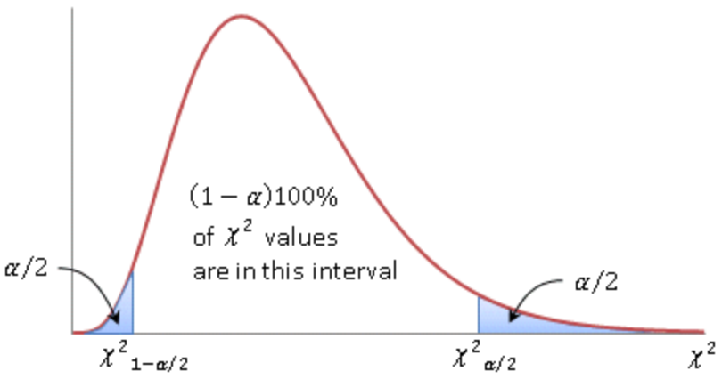
A less common way is to find a horizontal line such that the two resulting tail probabilities sum up to \(\alpha\).
CI for General Means
The Central Limit Theorem says the normalized sample mean converge in distribution to a standard normal random variable,
Hence, we have, approximately,
Rearranging the terms gives
Therefore,
is, approximately, a \(1-\alpha\) confidence interval for \(\mu\). The approximation is good if sample size \(n > 30\)
If \(\sigma\) is unknonw, then replace it by \(S\).
One-sample Mean Tests
The most common test is to test the mean of a given sample of observations.
The null hypothesis is \(H_0: \mu = \mu_0\). The alterntive hypothesis is \(H_1: \mu \ne \mu_0\) for a two-sided test, or \(H_1: \mu < \mu_0\) or \(H_1: \mu > \mu_0\) for one-sided tests.
Normal Means
Known Variance
Suppose the observations are from a normal distribution, \(X_i \overset{\text{iid}}{\sim} \mathcal{N} (\mu, \sigma^2)\) where \(\sigma^2\) is known. We have shown that
Hence, a test statistic can be
which follows a standard normal distribution under \(H_0\). The rejection region (RR) depends on the alternative hypoehtsis.
\(H_1\) |
RR |
RR if \(\alpha = 0.05\) |
|---|---|---|
\(\mu < \mu_0\) |
\(Z < - z_\alpha\) |
\(Z < - 1.645\) |
\(\mu > \mu_0\) |
\(Z > z_\alpha\) |
\(Z > 1.645\) |
\(\mu \ne \mu_0\) |
\(\left\vert Z \right\vert > z_{\alpha/2}\) |
\(\left\vert Z \right\vert > 1.960\) |
This is often known as a \(Z\)-test. But in practice, the population variance \(\sigma^2\) is unknown.
Unknown Variance
When \(X_i \overset{\text{iid}}{\sim} \mathcal{N} (\mu, \sigma^2)\) where \(\sigma^2\) is unknown, we have shown that
Hence, a test statistic can be
which follows a \(t_{n-1}\) distribution under \(H_0\). The rejection region (RR) depends on the alternative hypoehtsis.
\(H_1\) |
RR |
|---|---|
\(\mu < \mu_0\) |
\(T < - t_{n-1}^{\alpha}\) |
\(\mu > \mu_0\) |
\(T > t_{n-1}^{\alpha}\) |
\(\mu \ne \mu_0\) |
\(\left\vert T \right\vert > t_{n-1}^{\alpha/2}\) |
This is often known as a \(t\)-test.
General Means
By CLT, in for any distribution of \(X_i\), when the sample is large \((n \ge 30)\), we have
Hence a test statistic is
which approximately follows standard normal distribution. Then we use the usual \(Z\) test to decide the rejection regions.
For instance, if the null hypothesis is about a proportion \(H_0: p = p_0\), then we can model the random (binary) variable by a Bernoulli distribution \(X_i \sim \mathrm{Ber}(p_0)\) with mean \(p_0\) and variance \(p_0 (1-p_0)\). Therefore, the test statistic is
where \(\hat{p}\) is the observed proportion. A ususal \(Z\) test follows.
\(p\)-value Approach
Sometimes we can use the fundamental definition of \(p\)-value to compute it. Recall the definition is the probability of obtaining test results at least as extreme as the results actually observed, under the assumption that the null hypothesis is correct.
Binomial Distribution
We flip the coin 10 times and let \(X\) be the number of heads. Suppose we total number of heads \(X_{1}+\cdots+X_{10}=7\). Can we find the \(p\)-value for a test with rejection region of the form \(\{x \geq k\}\)
The observed value of the test statistic is \(\bar{X}=0.7\).
Since under the null hypothesis \(X=X_{1}+\cdots+X_{10} \sim \operatorname{Binomial}(10,0.5)\). Note the alternative hypothesis here is \(H_1: p > 0.5\).
For a two-sided test where \(H_1: p \ne 0.5\), the \(p\)-value is computed as
since ‘7 or more heads’ are as extreme as ‘3 or less heads’ under \(H_0\).
Geometric Distribution
Given \(X \sim \mathrm{Geo}(p)\), we can conduct a one-sided test
Let the observed value be \(k\). The \(p\)-value can be computed as
We then compare it with the significance level \(\alpha\) and draw a conclusion.
Alternatively, we can find a critical region by finding the integer \(j\) such that
If \(k \ge j\) then we reject \(H_0\). The actual significance level used here is \(\mathbb{P}(X \ge j \mid p=p_0)\).
Two-sample Mean Tests
Suppose we have two samples of data \(\left\{x_{1}, \cdots, x_{n}\right\}\) and \(\left\{y_{1}, \cdots, y_{m}\right\}\).
A question of interest: Did the two samples come from the same distribution, as opposed to, one sample having larger values than the other on average?
To model them, we assume
\(X_{i}, \cdots, X_{n}\) i.i.d. sampled from a distribution with mean with mean \(\mu_X\) and variance \(\sigma^2 _X\)
\(Y_{i}, \cdots, Y_{m}\) i.i.d. sampled from a distribution with mean with mean \(\mu_Y\) and variance \(\sigma^2 _Y\)
We are interested in comparing the two samples, often by comparing the two means \(\mu_X\) and \(\mu_Y\).
An unbiased estimator for the difference in mean \(\mu_X - \mu_Y\) is \(\bar{X} - \bar{Y}\). To provide standard error to this estimator, \(\operatorname{Var}\left( \bar{X} - \bar{Y} \right)\) need to be estimated, contingent on sample properties.
Paired
In many studies, the \(i\)-th measurements in the two samples \(x_i\) and \(y_i\) actually are related, such as measurements before and after a treatment from the same subject.
When \(m = n\) and \(\operatorname{Corr}\left( X_i,Y_i \right) = \rho \ne 0\), very often \(\rho >0\). Then,
To have a more precise variance estimate, it is appropriate to consider pairing \(X_i\) and \(Y_i\) by investigating their difference:
Note that \(D_i\)’s are i.i.d. under the i.i.d. assumption of each of the two samples, with
Then essentially, we changed the inference problem into that of a one-sample case.
An unbiased estimator for the variance of difference \(\sigma^2_D\) is the sample variance.
Normal
If \(X \sim \mathcal{N} \left(\mu_{X}, \sigma_{X}^{2}\right), Y \sim \mathcal{N} \left(\mu_{Y}, \sigma_{Y}^{2}\right)\), then we have the distributions for the sample estimators
In addition, they are independent. By the definition of \(t\)-distribution, the test statistic
is a pivot quantity not depending on the parameters if we are testing a hypothesis on \(\mu_D\). For instance,
A \((1-\alpha)\%\) confidence interval for the true difference in mean \(\mu_X - \mu_Y\) is
Non-normal
When the samples are not normally distributed, \(t_{n-1}\) can be used as an approximate distribution.
When n is large, we may use the Central Limit Theorem,
The asymptotic pivotal property can be used to conduct hypothesis tests.
A \((1-\alpha)\%\) confidence interval for the true difference in mean \(\mu_X - \mu_Y\) is
Independent
Now we consider \(X_i\) and \(Y_j\) are independent.
Equal Variance
If \(\sigma^2 _X = \sigma^2 _Y\), then
and both sample variances \(S_X^2\) and \(S_Y^2\) are unbiased estimators of \(\sigma^2\)
A better unbiased estimator is the pooled sample variance
which has a larger testing power than the two sample variances.
Normal
If both \(X\) and \(Y\) are of normal distributions, then the test statistic is
A \((1-\alpha)\%\) confidence interval for the true difference in mean \(\mu_X - \mu_Y\) is
Non-normal
When the samples are not normally distributed, \(t_{n+m-2}\) distribution can be used as an approximation.
When both \(n\) and \(m\) are large, we may apply the Central Limit Theorem,
Pooling vs paring
Consider the case n = m with equal variance.
Under assumption that the two samples are independent, the variance is
\[ \operatorname{Var}(\bar{X}-\bar{Y})= \frac{2 \sigma^{2}}{n} \]The pooled sample variance is the appropriate estimator to be used.
If the two samples were correlated with \(Corr(X_i, X_j) = \rho > 0\), the variance becomes smaller
\[ \operatorname{Var} (\bar{X}-\bar{Y})=(1-\rho) \frac{2 \sigma^{2}}{n}< \frac{2 \sigma^{2}}{n} \]
As a result, when correlation exists, the smaller paired sample variance is the appropriate one to use, since the test statistic using it has a larger power.
On the other hand, if the correlation is substantial and we fail to take it into consideration, the pooled sample variance estimator likely will overestimate the variance, and the estimate could be too large to be useful.
Unequal Variance
If \(\sigma_{X}^{2} \neq \sigma_{Y}^{2}\), the variance we are interested to estimate has the form
which can be estimated by the unbiased estimator
It is complicated to construct a pivot quantity like we did for the previous cases. Consider
When both \(X\) and \(Y\) are of normal distributions, we have
But since \(\sigma_{X}^{2} \neq \sigma_{Y}^{2}\), the summation
is not a multiple of a \(\chi^2\) distribution.
Hence, \(T\) is not \(t\)-distributed.
If \(n\) and \(m\) are both large, we can resort to Central Limit Theorem as usual,
The asymptotic approximation lead to a \((1-\alpha)\%\) confidence interval for the true difference in mean \(\mu_X - \mu_Y\)
However, there is a better approximation using \(t_v\) distribution than the normal approximation.
But the degree of freedom \(v\) is involved. It is estimated by Welch-Satterthwaite approximation,
The asymptotic approximation lead to a \((1-\alpha)\%\) confidence interval for the true difference in mean \(\mu_X - \mu_Y\),
Summary
The analysis for the above cases are summarized into the table below. In general, if \(X\) and \(Y\) are of normal distributions, the pivot quantity follows a known distribution. If not, we use CLT to obtain an approximate distribution, which requires large \(n\) and \(m\).
Dependency |
Test statistic |
Normal |
Non-normal, large \(n, m\) |
|---|---|---|---|
Paired (reduced to a univariate test) |
\(\frac{\bar{D}-\mu_{D}}{S_{D} / \sqrt{n}}\) |
\(\sim t_{n-1}\) |
\(\stackrel{\mathcal{D}}{\longrightarrow} \mathcal{N}(0,1)\) |
Independent with equal variance |
\(\frac{(\bar{X}-\bar{Y})-\left(\mu_{X}-\mu_{Y}\right)}{S_{p} \sqrt{\frac{1}{n}+\frac{1}{m}}}\) |
\(\sim t_{n+m-2}\) |
\(\stackrel{\mathcal{D}}{\longrightarrow} \mathcal{N}(0,1)\) |
Independent with unequal variance |
\(\frac{\left( \bar{X}-\bar{Y} \right)-\left(\mu_{X}-\mu_{Y}\right)}{\sqrt{\frac{S_{X}^{2}}{n}+\frac{S_{Y}^{2}}{m}}}\) |
/ |
\(\stackrel{\mathcal{D}}{\longrightarrow} t_v\) |
Multi-sample Mean Tests
Analysis of variance (ANOVA) is used to compare several univariate sample means. For instance, in the plot below, we have five levels and observed the response \(y\). We are interested in whether the five means are equal.
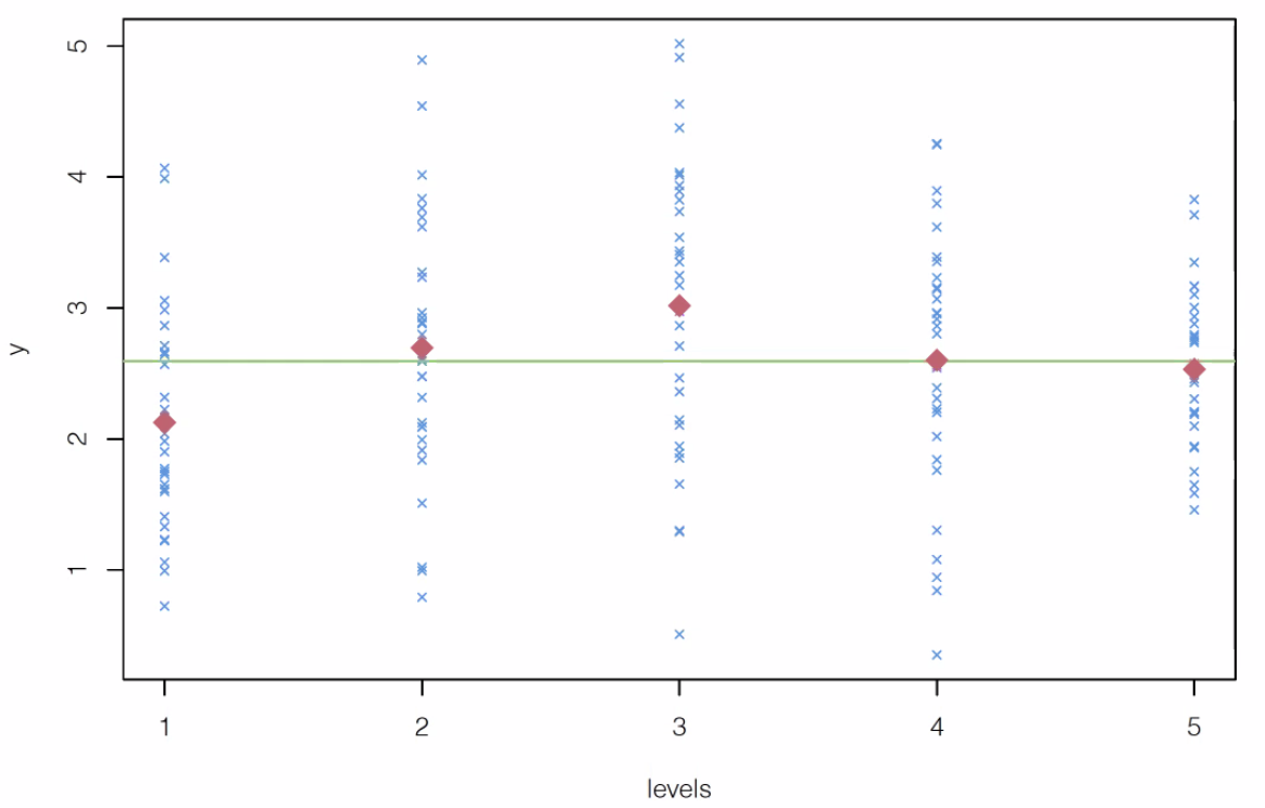
Fig. 27 One-way Layout
Model
There are \(n_\ell\) observations from population or treatment group \(\ell = 1, 2, \ldots, g\)
where
\(\mu\) is the overall mean parameter.
\(\tau_{\ell}\) is the treatment effect parameter of the \(\ell\) th population or \(\ell\) th treatment group.
\(e_{\ell j} \sim N\left(0, \sigma^{2}\right)\) is individual specific homogenous noise.
Parameter constraint: We have one \(\mu\) and \(g\) number of \(\tau_\ell\), in total \(1 + g\) parameters. There should be a constraint on the parameters such as \(\sum_{\ell=1}^{g} n_{\ell} \tau_{\ell}=0\), to avoid redundancy or unidentifiability.
To detect differences in treatment effects among the groups, the first test of interest is
Equivalently, the model can be parameterized as \(X_{\ell j} = \mu_\ell + e_{\ell j}\) without any parameter constraint, and the null hypothesis of equal treatment effects becomes equal means \(H_0: \mu_1 = \ldots = \mu_g\).
Test Statistic
First, we decompose the observations as
where \(\bar{x}\) is the overall mean, \(\bar{x}_\ell\) is the \(\ell\)-th group mean. Hence, the observation can be seen as estimated overall mean + estimated treatment effect + estimated noise. Equivalently,
Summing up all squared terms, noticing that \(\sum_{\ell=1}^{g} \sum_{j=1}^{n_{\ell}}\left(\bar{x}_{\ell}-\bar{x}\right)\left(x_{\ell j}-\bar{x}_{\ell}\right)=0\), we have
The decomposition can be stated as
The corresponding numbers of independent quantities of each term, i.e. the degrees of freedom, have the relation
Therefore, we obtain the analysis of variance table
At test level \(\alpha\), the null \(H_0: \tau_{1}=\cdots=\tau_{g}=0\) is rejected if
Cavests in using anova()
In anova() function in R, if the group variable \(\ell\) is in numerical value, it is necessary to coerce it as data type factor by calling as.factor().
When \(g=2\), the ANOVA \(F\)-test reduces to the two-sample means \(t\)-test.
The null hypothesis is equal means \(H_0: \mu_1 = \mu_2\)
The test statistic have the relation \(t^2 = F\).
The two \(p\)-values are the same.
Multivariate Settings
Hotelling’s \(T^2\) Distribution
- Definition (Hotelling’s \(T^2\) Distribution )
Suppose random zero-mean Gaussian \(\boldsymbol{x} \sim \mathcal{N} _p(\boldsymbol{0} , \boldsymbol{\Sigma} )\) and Wishart random matrix \(\boldsymbol{V} \sim W_p(k, \boldsymbol{\Sigma} )\) are independent. Define
\[ T^2 = k \boldsymbol{x} ^{\top} \boldsymbol{V} ^{-1} \boldsymbol{x} \]Then \(T^2\) is said to follow a Hotelling’s \(T^2\) distribution with parameter \(p\) and \(k\), denoted as \(T^2(p, k)\).
In univariate sense, the Hotelling’s \(T^2\) statistic can be reduced to the squared \(t\)-statistic. Hence it can be seen as multivariate generalization of (squared) \(t\)-distribution.
- Properties
If \(\bar{\boldsymbol{x}}\) and \(\boldsymbol{S}\) are respectively the sample mean vector and sample covariance matrix of a random sample of size \(n\) taken from \(\mathcal{N} _p(\boldsymbol{\mu} , \boldsymbol{\Sigma} )\), then
\[n(\bar{\boldsymbol{x}}-\boldsymbol{\mu})^{\top} \boldsymbol{S}^{-1}(\bar{\boldsymbol{x}}-\boldsymbol{\mu}) \sim T^{2}(p, n-1)\]The distribution of the quadratic form under non-normality is reasonably robust as long as the underlying multivariate distribution has pdf contours close to elliptical shape, but \(T^2\) is sensitive to the departure from such elliptical symmetry of the distribution.
Invariant under transformation of \(\boldsymbol{x}\):\(\boldsymbol{C} \boldsymbol{x} + \boldsymbol{d}\), where \(\boldsymbol{C}\) is non-singular.
Related to other distribution:
\(T^{2}(p, k)=\frac{k p}{k-p+1} F(p, k-p+1)\), usually used to find quantile \(T^2(\alpha)\).
\(T^{2}(1, k)=t^{2}(k)=F(1, k)\)
\(T^{2}(p, \infty) \rightarrow \chi ^2 _p\) by multivariate CLT, without assuming normality of the distribution of \(\boldsymbol{x}\)
Related to Mahalanobis distance: \(T^{2}=n D_{\boldsymbol{S}}^{2}(\bar{\boldsymbol{x}}, \boldsymbol{\mu})\)
One-sample Mean
Assume \(\boldsymbol{x} \sim \mathcal{N} _p(\boldsymbol{0} , \boldsymbol{\Sigma} )\), want to test
- Test statistic under \(H_0\)
\(\boldsymbol{\Sigma}\) is known:
\[T^{2}=n\left(\bar{\boldsymbol{x}}-\boldsymbol{\mu}_{0}\right)^{\top} \boldsymbol{\Sigma}^{-1}\left(\bar{\boldsymbol{x}}-\boldsymbol{\mu}_{0}\right) \sim \chi^{2}(p)\]\(\boldsymbol{\Sigma}\) is unknown, estimated by \(\boldsymbol{S}\):
\[\begin{split}\begin{aligned} T^{2}=n\left(\bar{\boldsymbol{x}}-\boldsymbol{\mu}_{0}\right)^{\top} \boldsymbol{S}^{-1}\left(\bar{\boldsymbol{x}}-\boldsymbol{\mu}_{0}\right) &\sim T^{2}(p, n-1) \\ &\sim \frac{(n-1) p}{n-p} F(p, n-p) \\ & \rightarrow \chi ^2 _p \quad \text{as } n \rightarrow \infty \end{aligned}\end{split}\]Analogously, in univariate case,
\[\begin{split} \left\{\begin{array}{l} \frac{\sqrt{n}\left(\bar{x}-\mu_{0}\right)}{\sigma} \sim N(0,1) \text { if } \sigma^{2} \text { is known } \\ \frac{\sqrt{n}\left(\bar{x}-\mu_{0}\right)}{s} \sim t(n-1) \text { if } \sigma^{2} \text { is unknown. } \end{array}\right. \end{split}\]
- Confidence Region
A \((1-\alpha)100\%\) confidence region for \(\boldsymbol{\mu}\) is a \(p\)-dimensional ellipsoid centered at \(\bar{\boldsymbol{x}}\), i.e. a collection of all those \(\boldsymbol{\mu}\) which will not be rejected by the above \(T^2\) test at significance level \(\alpha\).
\[ \left\{\boldsymbol{\mu}: n(\bar{\boldsymbol{x}}-\boldsymbol{\mu})^{\top} \boldsymbol{S}^{-1}(\bar{\boldsymbol{x}}-\boldsymbol{\mu}) \leq T_{\alpha}^{2}(p, n-1)=c_{\alpha}\right\} \]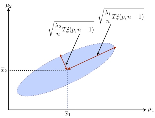
Fig. 28 Confidence region
This confidence ellipsoid above is the most precise confidence region of the vector \(\boldsymbol{\mu}\), in the sense that any other form of confidence region for \(\boldsymbol{\mu}\) with the same confidence level \((1-\alpha)\) will have larger volume in the \(p\)-dimensional space of \(\boldsymbol{\mu}\) and hence less precise.
- Simultaneous confidence intervals for each component
Individual CIs: Sometimes people get used to confidence intervals for individual components, such as
\[ \bar{x}_{j}-t^{\alpha / 2}_{n-1} \frac{s_j}{\sqrt{n}} <\mu_{j}<\bar{x}_{j}+t^{\alpha / 2}_{n-1} \frac{s_j}{\sqrt{n}} \]where \(\bar{x}_j\) and \(s_j\) are respectively the sample mean and standard deviation of the \(j\)-th variate that has mean \(\mu_j\). But there are multiple testing issues. We can then use Bonferroni or Scheffe simultaneous C.I.s to correct this.
The \((1-\alpha)100\%\) Bonferroni simultaneous C.I.s for \(m\) pre-determined linear components of means, \(\boldsymbol{a}_{i}^{\top} \boldsymbol{\mu}(i=1, \ldots, m)\), are given by
\[ \boldsymbol{a}_{i}^{\top} \bar{\boldsymbol{x}} \pm t ^{\alpha/(2m)}_{n-1} \sqrt{\frac{\boldsymbol{a}_{i}^{\top} \boldsymbol{S} \boldsymbol{a}_{i}}{n}} \]
The \((1-\alpha)100\%\) Scheffe simultaneous C.I.s for all possible linear combinations of means \(\boldsymbol{a} ^{\top} \boldsymbol{\mu}\) are given by
\[ \boldsymbol{a}^{\top} \bar{\boldsymbol{x}} \pm \sqrt{T_{\alpha}^{2}(p, n-1)} \sqrt{\frac{\boldsymbol{a}^{\top} \boldsymbol{S a}}{n}} \]Pros: Compared with the advantages of ellipsoidal confidence regions, these hyper-rectangles (orthotopes) are easier to form and to compute.
Cons: Both Bonferroni and Scheffé intervals are wider (hence less accurate) than the ordinary confidence intervals which are constructed with separate confidence level of \((1-\alpha)\).
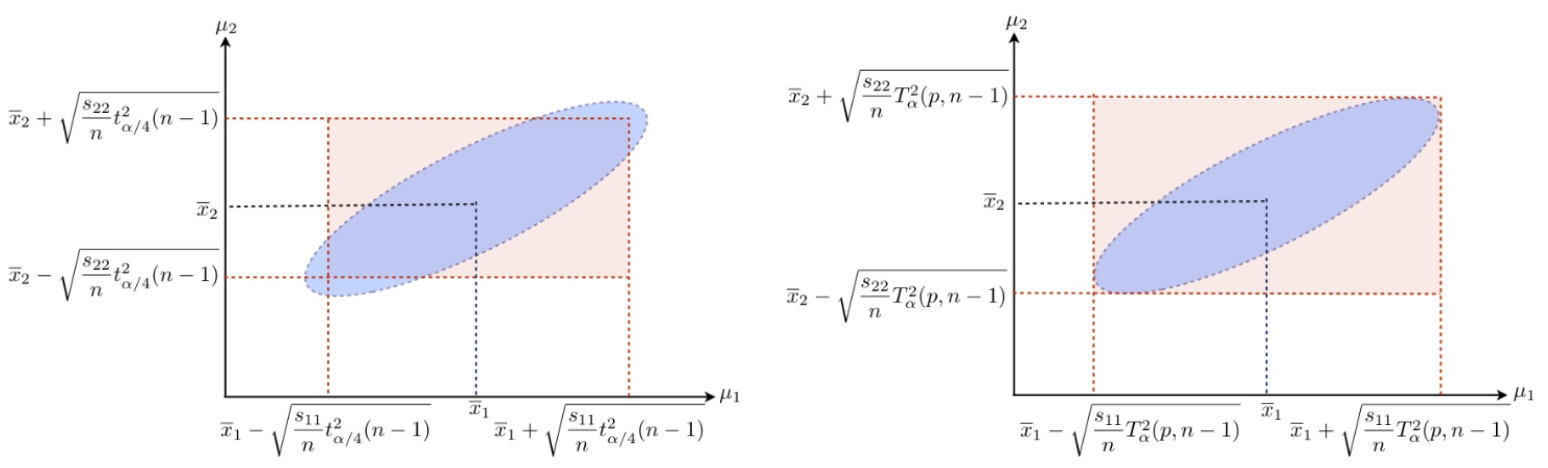
Fig. 29 Bonferroni (left) and Scheffe (right) simultaneous C.I.s.
If we just want to conduct univariate tests of means \(H_0: \mu_k = 0\) for each \(k = 1, 2, \ldots, p\), i.e. \(\boldsymbol{a} _k = \boldsymbol{e} _k\), then the C.I. has the general form \(\bar{x}_{k} \pm c_{n, p, \alpha} \sqrt{\frac{s_{k k}}{n}}\) for some multiplier \(c_{n, p, \alpha}\) depending on \(n,p,\alpha\). The above methods can be summarized as follows
marginal C.I. using \(t\) statistics (ignoring dependence among components): \(t_{n-1}^{\alpha/2}\)
Bonferroni simultaneous C.I. using \(t\) statistics: \(t_{n-1}^{\alpha/(2p)}\)
Scheffe simultaneous C.I.: \(\sqrt{T^2_\alpha (p, n-1)}\)
Asymptotic simultaneous C.I. using \(\chi ^2\) statistic as \(n\) is large: \(\sqrt{\chi ^2 _p (\alpha)}\)
Two-sample Means
Given two samples of \(p\)-variates, we are interest in whether their means are equal.
Paired
First, we consider paired comparison for two dependent samples.
This is easy, we just define \(\bar{\boldsymbol{d}} = \bar{\boldsymbol{x}}_1 - \bar{\boldsymbol{x}}_2\), and apply the above one-sample mean method to test \(H_0: \boldsymbol{d} = \boldsymbol{0}\).
More precisely, if \(\boldsymbol{d} \sim \mathcal{N} _p (\boldsymbol{\delta}, \boldsymbol{\Sigma} _d)\)
Two Independent Samples
We assume equal variance \(\boldsymbol{\Sigma} _1 = \boldsymbol{\Sigma} _2 = \boldsymbol{\Sigma}\). The pooled sample covariance matrix is an unbiased estimator of it
By the independence between the two samples, the covariance of sample difference is
which can be estimated by \(\left(\frac{1}{n_{1}}+\frac{1}{n_{2}}\right) \boldsymbol{S}_{\text {pool }}\) since
Assume \(\boldsymbol{x} _1 \sim \mathcal{N} _p (\boldsymbol{\mu} _1, \boldsymbol{\Sigma} ), \boldsymbol{x} _2 \sim \mathcal{N} _p (\boldsymbol{\mu} _2, \boldsymbol{\Sigma} )\), then under \(H_0: \boldsymbol{\mu} _1 = \boldsymbol{\mu} _2\),
where
The \((1-\alpha)\%\) Bonferroni simultaneous confidence interval for the difference of the \(j\)-th component means \(\mu_{1j} - \mu_{2j}\) is
More generally,
\((1-\alpha)\%\) Bonferroni intervals for pre-determined \(\boldsymbol{a}_{i}^{\top}\left(\boldsymbol{\mu}_{1}-\boldsymbol{\mu}_{2}\right), i=1, \ldots, k\) is
\[ \boldsymbol{a}_{i}^{\top}\left(\bar{\boldsymbol{x}}_{1}- \bar{\boldsymbol{x}}_{2}\right) \pm t_{n_{1}+n_{2}-2}^{\alpha / (2 k)} \sqrt{\left(\frac{1}{n_{1}}+\frac{1}{n_{2}}\right)\boldsymbol{a}_{i}^{\top} \boldsymbol{S}_{\text{pool} } \boldsymbol{a}_{i}} \]\((1-\alpha)\%\) Scheffe simultaneous intervals for \(\boldsymbol{a}^{\top}\left(\boldsymbol{\mu}_{1}-\boldsymbol{\mu}_{2}\right)\) for all \(\boldsymbol{a}\) is
\[ \boldsymbol{a}^{\top}\left(\bar{\boldsymbol{x}}_{1}- \bar{\boldsymbol{x}}_{2}\right) \pm \sqrt{T_{\alpha}^{2}\left(p, n_{1}+n_{2}-2\right)} \sqrt{\left(\frac{1}{n_{1}}+\frac{1}{n_{2}}\right)\boldsymbol{a}^{\top} \boldsymbol{S}_{\text{pool} } \boldsymbol{a}} \]
MANOVA
If there are multiple samples of multivariate observations, we use Multivariate Analysis of Variance (MANOVA). The data are treated as \(g\) sample groups of observed sample values, each sample group is from one of \(g\) populations.
Model
The MANOVA model, generalized from ANOVA, becomes
\(\boldsymbol{\mu}\) is the overall mean vector,
\(\boldsymbol{\tau} _{\ell}\) is the treatment effect vector of the \(\ell\) th population or treatment group,
\(\boldsymbol{e}_{\ell j} \sim N_{p}(0, \Sigma)\) is individual specific homogenous noise.
The parameter constraint here is \(\sum_{\ell=1}^{g} n_{\ell} \boldsymbol{\tau}_{\ell}=0\).
Analogous to the univariate case, the test of interest is
Equivalently, the model can be parameterized as \(\boldsymbol{x}_{\ell j} = \boldsymbol{\mu}_\ell + \boldsymbol{e}_{\ell j}\) without any parameter constraint, and the null hypothesis of equal treatment effects becomes equal means \(H_0: \boldsymbol{\mu} _1 = \ldots = \boldsymbol{\mu} _g\).
Test Statistic
The data can be decomposed similarly,
or
Then
Summing up, we have
since
The decomposition can be stated as
with corresponding degrees of freedom
Now we analyze the test statistic
Denote the between group (or between population) sum of squares and cross products matrix as
and the within group sum of squares and cross products matrix as
In fact \(\boldsymbol{W}\) is related to the pooled covariance matrix,
The MANOVA table is then
Since \(\boldsymbol{B}\) and \(\boldsymbol{W}\) are \(p \times p\) covariance matrices, the test statistic uses their determinants, or the generalized variances.
We introduce Wilks’ Lambda
which is the ratio of generalized variance of residual / generalized variance of total.
The distribution of \(\Lambda^{*}\) depends on \(p, g, n_\ell\) and is related to \(F\) distribution. When \(n = \sum n_\ell\) is large, Bartlett gives a simple chi-square approximation
Even for moderate sample size, it is good practice to check and compare both tests.
Note
We reject the null hypothesis that all group means are equal if the value of \(\Lambda^{*}\) is too “small”.
Wilks’ lambda is equivalent to the likelihood ratio test statistic.
Under the null Wilks’ lambda is of its own \(\Lambda^{*}\)-distribution, which is derived from the ratio of two random matrices \(\boldsymbol{W}\) and \(\boldsymbol{B} + \boldsymbol{W}\), each is of Wishart distribution
We can express Wilks’ lambda by eigenvalues of \(\boldsymbol{B} \boldsymbol{W} ^{-1}\), which can be seen as signal-noise ratio. If it is large, then \(\lambda\) is large, and \(\Lambda^{*}\) is small.
\[ \Lambda^{*}=\frac{|\boldsymbol{W}|}{|\boldsymbol{B}+\boldsymbol{W}|}=\frac{1}{\left|\boldsymbol{W}^{-1} \boldsymbol{B}+\boldsymbol{I}\right|}=\prod_{k=1}^{p} \frac{1}{1+\lambda_{k}} \]The 2nd equality holds due to \(\operatorname{det}(\boldsymbol{X} \boldsymbol{Y} ) = \operatorname{det}(\boldsymbol{X} ) \operatorname{det} (\boldsymbol{Y})\). Note that since \((\boldsymbol{B} \boldsymbol{W} ^{-1} )^{\top} = \boldsymbol{W} ^{-1} \boldsymbol{B}\), the two matrices \(\boldsymbol{B} \boldsymbol{W} ^{-1}\) and \(\boldsymbol{W} ^{-1} \boldsymbol{B}\) share the same eigenvalues.
Other test statistics using the eigenvalues of \(\boldsymbol{B} \boldsymbol{W} ^{-1}\) include
Hotelling-Lawley’s Trace: \(\operatorname{tr}\left(\mathbf{B W}^{-1}\right)=\sum_{k=1}^{p} \lambda_{k}\)
Pillai’s Trace: \(\operatorname{tr}\left(\boldsymbol{B}(\boldsymbol{B}+\boldsymbol{W})^{-1}\right)=\operatorname{tr}\left(\boldsymbol{B} \boldsymbol{W}^{-1}\left(\boldsymbol{B} \boldsymbol{W}^{-1}+\boldsymbol{I} \right)^{-1}\right)=\sum_{k=1}^{p} \frac{\lambda_{k}}{1+\lambda_{k}}\)
Roy’s Largest Root: \(\max _{k}\left\{\lambda_{k}\right\}=\left\|\boldsymbol{B} \boldsymbol{W}^{-1}\right\|_{\infty}\) which gives an upper bound.
C.I. for Difference in Two Means
If the null hypothesis of MANOVA is rejected, a natural question is, which treatments have significant effects?
To compare the effect of treatment \(k\) and treatment \(\ell\), the quantity of interests is the difference of the vectors \(\boldsymbol{\tau}_k - \boldsymbol{\tau}_\ell\) which is the same as \(\boldsymbol{\mu} _k - \boldsymbol{\mu} _\ell\). For two fixed \(k, \ell\), there are \(p\) variables to compare. For each variable \(i\), we want a confidence interval for \(\tau_{ki} - \tau_{\ell i}\), which have the form
where the multiplier \(c\) depends on the level and the type of the confidence interval.
Assuming mutual independence and equal variance \(\boldsymbol{\Sigma}\) among the \(g\) samples, using Bonferroni correction, we have
\(c = t_{n-g}^{\alpha/2m}\), where \(m= p \binom{g}{2}\) is the number of simultaneous confidence intervals.
\(\widehat{\operatorname{Var}}\left(\hat{\tau}_{k i}-\hat{\tau}_{\ell i}\right)=\frac{w_{i i}}{n-g}\left(\frac{1}{n_{k}}+\frac{1}{n_{\ell}}\right)\) where \(w_{ii}\) is the diagonal entry of \(\boldsymbol{W}\).
Note that
The Bonferroni method often gives confidence intervals too wide to be practical even for moderate \(p\) and \(g\).
The equal variance can be tested.
Test for Equal Covariance
Are the variables in the \(g\) population groups sharing the same covariance structure?
Box’s \(M\)-test for equal covariance structure is a likelihood-ratio type of test. Denote
where
Box’s test is based on an approximation that the sampling distribution of \(\ln \Lambda\) is approximately of \(\chi ^2\) distribution under the equal covariance matrix hypothesis. Box’s \(M\) is defined as
Under the hypothesis \(H_0\) of equal covariance, approximately
where
\(u = \left(\sum_{\ell=1}^{g} \frac{1}{n_{\ell}-1}-\frac{1}{n-g}\right) \frac{2 p^{2}+3 p-1}{6(p+1)(g-1)}\)
\(v = p(p+1)(g-1)/2\)
\(H_0\) is rejected if \((1-u) M > \chi_{v}^{2}(\alpha)\). Box’s M-test works well for small \(p\) and \(g\) \((\le 5)\) and moderate to large \(n_\ell\) \((\ge 20)\).