Self-supervised Learning
In supervised learning, we have \(\left(\boldsymbol{x}_{i}, y_{i}\right)\) and an objective \(\min \sum_{i} L\left(f\left(\boldsymbol{x}_{i}, \theta\right), y_{i}\right)\).
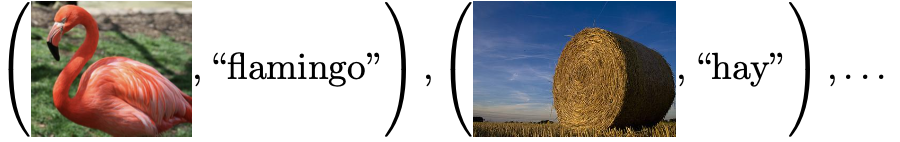
Fig. 44 Data \((\boldsymbol{x} _i, y_i)\) in supervised learning [Shakhnarovich 2021]
In unsupervised learning, we only have \(\boldsymbol{x} _i\), the objective is specified as a function of \((\boldsymbol{x} _i, f(\boldsymbol{x} _i))\), e.g. clustering, dimensionality reduction.
In self-supervised learning, data comes in form of multiple channels \((\boldsymbol{x}_i ,\boldsymbol{z}_i )\). Our goal is to predict \(\boldsymbol{z}\) from \(\boldsymbol{x}\). This is similar to supervised learning, but with no manual labels \(y_i\), and \(\boldsymbol{z}\) is inherent in data. The \(\boldsymbol{z}\) here are some “proxy” or “pretext”. In order to predict it well, the model need to have a good understanding/representation of \(\boldsymbol{x}\).
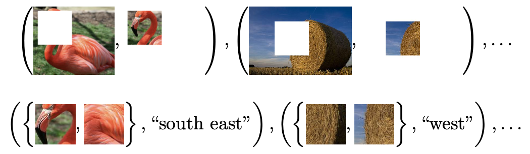
Fig. 45 Data \((\boldsymbol{x} _i, \boldsymbol{z} _i)\) in self-supervised learning [Shakhnarovich 2021]
Proxy Task
Proxy tasks include
Colorization
Color gray scale images
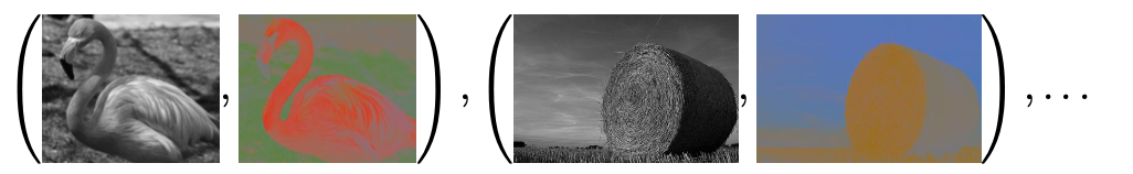
Fig. 46 Colorization [Shakhnarovich 2021]
Inpainting (mask reconstruction)
Fill a masked part in an image
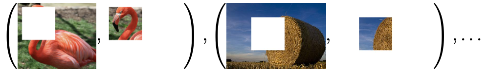
Fig. 47 Inpainting [Shakhnarovich 2021]
Given two patches of an image, determine their relative position.
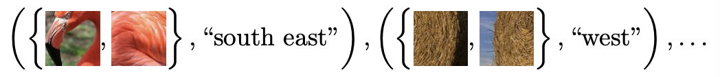
Fig. 48 Relative position [Shakhnarovich 2021]
Solving jigsaw puzzles
Learn to identify more probable permutations of image pieces
Learn to predict soundtrack (more precisely, a cluster to which the soundtrack should be assigned) from a single video frame [Owens et al., 2016]
Predicting video frame from previous frames
Contrastive Learning
“Simple framework for Contrastive Learning of visual Representations” (Chen et al., 2020)
Consider pairs of views from the same image. Goal is to maximize similarity for matching pairs and dissimilarity for non-matching pair
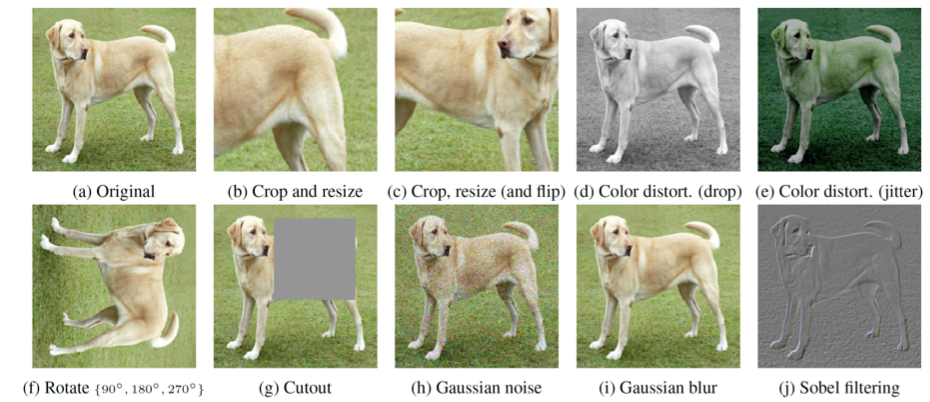
Fig. 49 Views (transformations)
Computation graph:
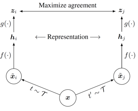
Fig. 50 Computational graph of contrastive learning
Contrastive Predictive Coding
For objects of spatial or temporal order.
Idea :
Predictive coding means the coding is capable to predict some learned representation of other parts of the object.
In these reconstruction tasks, some layers in the model can be regarded as the learned representation of the image/text/speech, which can be used for downstream tasks.
For Speech (Wav2vec)
Speech: predict future speech segments
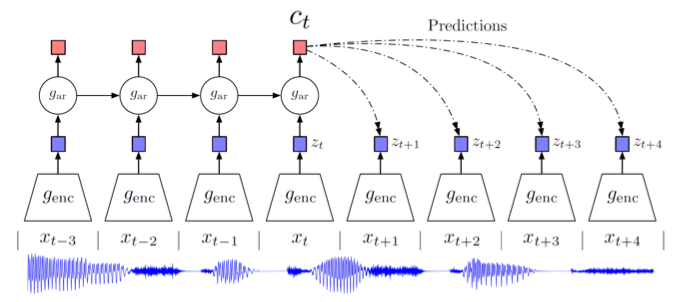
Fig. 51 CPC for speech
\(x_t\) is input
\(z_t\) is representation of \(x_t\)
\(c_t\) is more high-level contextual coding for predicting future representation \(z_{t+1}, z_{t+2}, \ldots\) since predicting the actual \(x_t\) might be too hard or not useful.
Contrastive Loss \(\mathcal{L} = \sum_{k=1}^K \mathcal{L}_k\), where
where
\(h_k(\boldsymbol{c}_i)\) is the predicted future representation, and \(\sigma(\boldsymbol{z} _{i+k} ^{\top} h_k(\boldsymbol{c}_i))\) is a probability-like similarity measure. We want to maximize this quantity.
the second part, we randomly draw \(\tilde{\boldsymbol{z} }\) from other far away time steps, and minimize the similarity between this negative example and the predicted representation.
want to learn a representation that can differentiate true future step and distractors.
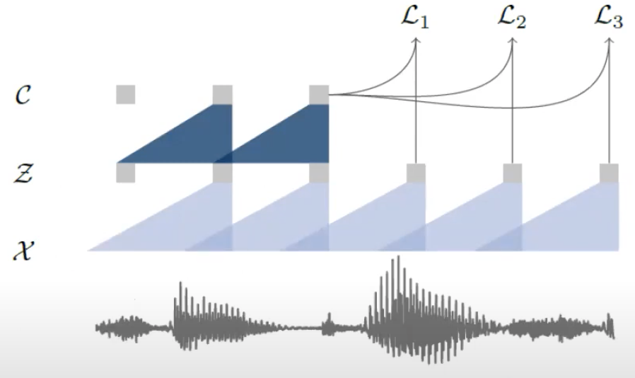
Fig. 52 Contrastive Loss [Schneider et al. 2019]
Wav2vec 2.0 add a quantized representation layer. Predict masked window.
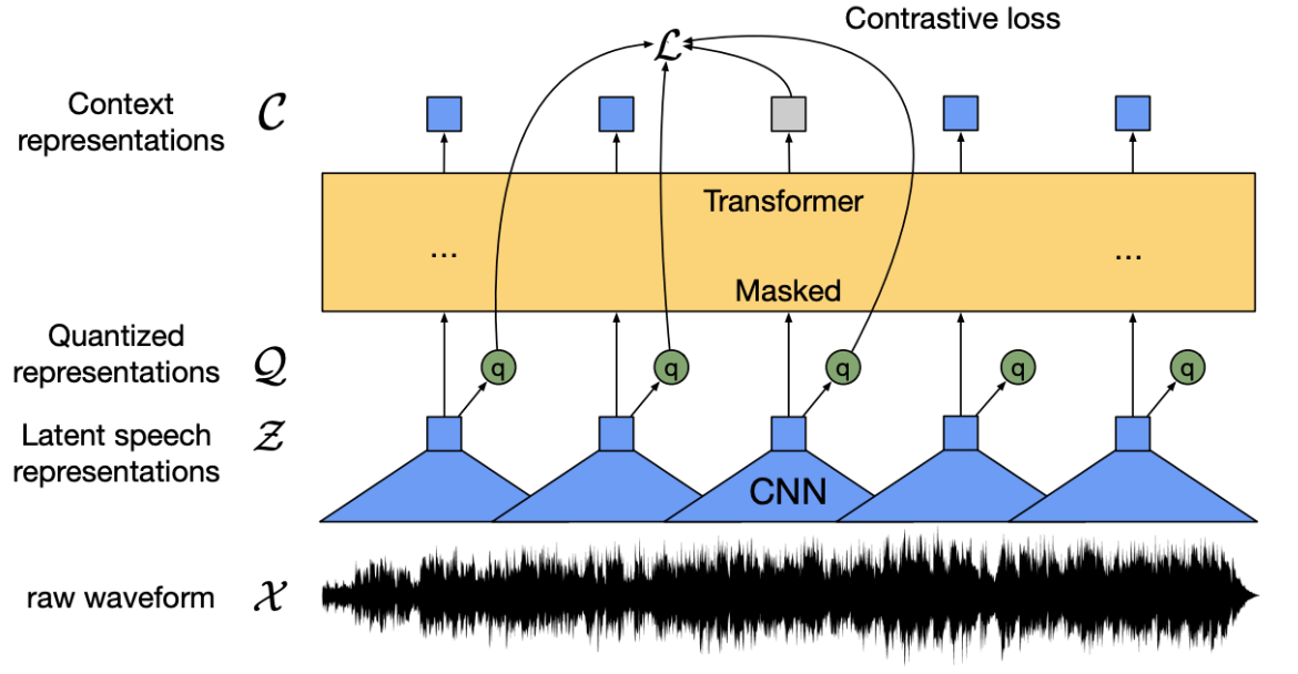
Fig. 53 Wav2vec 2.0 [Baevski et al. 2020]
For Vision
Predict some part of the image from another part
Encode image patches (using CNN)
Predict, from the context embedding of the patches above some level, a patch below that level
Actual embedding of the patch \(\boldsymbol{z} _i\), predicted \(\hat{\boldsymbol{z}}_i\)
Loss for patch \(i\)
\[ -\log \frac{\widehat{\boldsymbol{z}}_{i} \cdot \boldsymbol{z}_{i}}{\widehat{\boldsymbol{z}}_{i} \cdot \boldsymbol{z}_{i}+\sum_{n} \widehat{\boldsymbol{z}}_{i} \cdot \boldsymbol{z}_{n}} \]where \(n\) goes over (sampled) other patches, both in this image and in other images
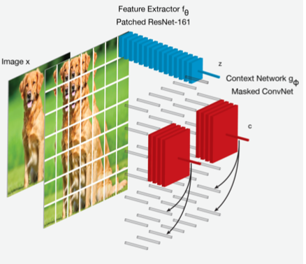
Fig. 54 CPC for image
Others
CLIP: Learning Transferable Visual Models From Natural Language Supervision (OpenAI, 2021)