Graph Basics
A graph \(G = (V, E)\) contains vertex set \(V\) and edge set \(E\), with size \(\left\vert V \right\vert = N_v\) and order \(\left\vert E \right\vert = N_e\).
In particular, \(E\) is a 2-subset of \(V\).
Vertex- and Edge-level Concepts
Connectivity
If there is and edge \((u, v)\) connecting vertices \(u\) and \(v\), we say \(u\) are \(v\) are ends of edge \(e\), or \(u\) and \(v\) are adjacent, or neighbors.
If two edges \(e_1 = (u, v)\) and \(e_2 = (u, w)\) shares a common vertex \(u\), we say \(e_1\) and \(e_2\) are adjacent.
If a vertex is an endpoint of an edge \(e\), we say \(v\) is incident on \(e\).
Neighborhood of a vertex: The (open) neighborhood of a vertex \(v\) in graph \(G\) is \(N_G(v)= \left\{ u \mid (u, v) \in E(G) \right\}\). The closed neighborhood is \(N_G [v] = N_G(v) \cup \left\{ v \right\}\).
Degree of a vertex: The degree of a vertex \(v\) is the number of its neighbors. \(\operatorname{deg}_G (v) = \left\vert N_G(v) \right\vert\). In short we write \(d_v\).
Minimum degree is denoted as \(\delta(G)=\min _v \operatorname{deg}_G(v)\)
Maximum degree is denoted as \(\Delta(G)=\max _v \operatorname{deg}_G(v)\)
Sum of degree: \(\sum _{v \in V} \operatorname{deg}_G(v) = 2 N_e\)
Corollary: In any graph, there are an even number of odd-degree vertices.
Degree sequence of a graph is the sequence formed by arranging the vertex degree \(d_v\) in non-decreasing order.
For digraphs, vertex degree is replaced by in-degree \(d_v^{in}\) and out-degree \(d_v ^{out}\).
Havel-Hakimi theorem
Path: A path \(P_n\) is a graph whose vertices can be arranged in a sequence \((v_1, \ldots, v_n)\) such that the edge set is \(E = \left\{ (v_i, v_{i+1}) \mid i=1, \ldots, n-1 \right\}\).
Cycle: A cycle \(C_n\) is a graph whose vertices can be arranged a cycle sequence \((v_1, v_2, \ldots, v_n)\) such that the edge set is \(E = \left\{ (v_i, v_{i+1}) \mid i=1, \ldots, n-1 \right\} \cup \left\{ (v_n, v_1) \right\}\).
A graph with no cycles is called acyclic.
The girth of an undirected graph is the length of a shortest cycle contained in the graph. If the graph does not contain any cycles (that is, it is a forest), its girth is defined to be infinity
If in a graph \(G\), all vertices have degree at least 2, then \(G\) contains a cycle.
Proof
Let \(P=(v_0, \ldots, v_{k})\) be a longest path in \(G\). Since \(\operatorname{deg} (v_k) \ge 2\), then there is a vertex \(v \in V, v \ne v_{k-1}\), such that \(v\) is adjacent to \(v_k\). If \(v \notin P\), then we have a longer path in \(G\), contradiction. Hence, \(v \in P\). More precisely, \(v = v_i\) for some \(0\le i \le k-2\). Thus, \(v_k\) is connected to two vertices in \(P\), which forms a cycle.
Walk: A walk in a graph \(G\) is a sequence \(W=(v_0, e_1, v_1, e_2, \ldots, v_{k-1}, e_k, v_k)\) whose terms alternate between vertices and edges (not necessarily distinct) such that \(v_{i-1} v_i = e_i\) for \(1 \le i \le \ell\). When \(G\) is simple, we may write the walk by indicating the vertices only.
A walk is closed if the start and end vertices are the same \(v_0 = v_k\).
A path is a walk such that all of the vertices and edges are distinct. If there is a walk from \(u\) to \(v\), then there is a path from \(u\) to \(v\) by removing all cycles in the walk.
The length of a walk is the number of edges of the walk. If is a walk from \(x\) to \(y\) of length \(k\), we write \(x \overset{k}{\rightarrow} y\). If \(k\) is unknown, we write \(x \overset{\star}{\rightarrow} y\).
A vertex \(v\) is reachable from another vertex \(u\) if there exists a walk from \(u\) to \(v\).
Trail: A trail is a walk such that all of the edges are distinct.
An Euler trail visits every edge once. A graph has a Euler trail if and only if the number of odd-degree nodes are 0 or 2. Moreover, if 0, then and node can be the start node, as well as the end node. If 2, then the two nodes are start and end nodes.
An Euler tour is an Euler trail that is closed. If a graph has an Euler tour, we call it Eulerian. A graph \(G\) is Eulerian if and only if every vertex of \(G\) has even degree.
Circuit: A trail for which the beginning and ending vertices are the same.
(Geodesic) Distance between two vertices: The distance between two vertices \(u\) and \(v\) in \(G\) is the minimal length of a walk from \(u\) to \(v\). \(\operatorname{dist} (u,v) = \min \left\{ k \mid u \overset{k}{\rightarrow} v \right\}\). If there is no walk, then the distance is \(\infty\).
Diameter of a graph is the longest distance in a graph: \(\operatorname{diam} (G) = \max_{u,v \in V} \operatorname{dist} (u,v)\)
Families of Graphs
Self-edge (self-loops): allow self-edge \((u,u)\)
Multi-graph: allow multiple edges between two vertices.
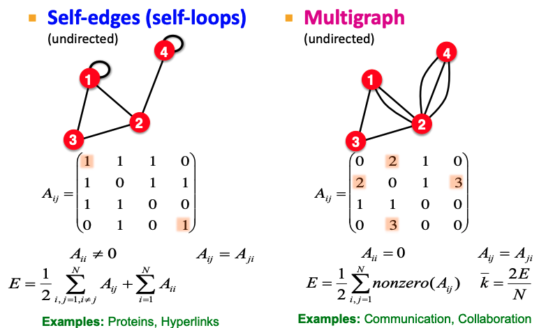
Fig. 192 Self-edges graph and multigraph
Simple graph: no self-edges, and no multiple edges.
Directed graph: directed edges called arcs.
Two arcs \((u, v)\) and \((v, u)\) are said to be mutual.
Multi-digraphs: multiple arcs share the same head and tail.
Connected graph: There is a path between every pairs of vertices.
Bridge edge: an edge \(e \in E(G)\) is a bridge of \(G\) if \(G \setminus e\) has more connected components than \(G\). In particular, if \(G\) is connected, then \(G \setminus\) is disconnected.
An edge \(e \in E(G)\) is a bridge if and only \(e\) is not in any cycle of \(G\).
Articulation node: if we erase the node, the graph becomes disconnected.
The maximal connected subgraphs of \(G\) are its connected components. We use \(c(G)\) to denote the number of connected components in \(G\). If \(c(G)=1\) then \(G\) is connected. “Maximal” here means if we add any one of other vertex to the connected subgraph, it becomes disconnected.
To identify connectivity, we can check the adjacency matrix. The adjacency matrix of a graph with several components can be written in a block-diagonal form, so that nonzero elements are confined to squares, with all other elements being zero.
Connected directed graph:
Strong connected: has a path from each node to every other node and vice versa (\(a \rightarrow b\) and \(b \rightarrow a\)).
Weakly connected: connected if we disregard the edge directions.
Strongly connected components: a component that is strongly connected.
in-component: nodes that can reach SCC
out-component: nodes that can be reached from SCC
Completed graph: every pair of vertices are adjacent, denoted as \(K_n\), where \(n=\left\vert V \right\vert\).
Clique: A complete subgraph. It is a maximal clique if no other clique contains it.
Empty graph: no edges, \(E = \emptyset\).
An empty graph \(\Leftrightarrow\) a \(0\)-regular graph.
Bipartite graph: A graph whose vertex set can be partitioned into 2 sets \(U\) and \(V\) such that every edge \((u, v) \in E\) has \(u \in U\) and \(v \in V\). We usually write \(G=(U,V,E)\).
Characterization: A graph \(G\) is bipartite iff it contains no odd cycle.
Claims:
A path is bipartite.
A cycle is bipartite iff its has even length.
Property: \(\sum_{v \in V} \operatorname{deg}(v) = \sum_{u \in U} \operatorname{deg} (u) = \left\vert E \right\vert\)
Complete bipartite graph: \(E\) has every possible edge between the two sets \(U\) and \(V\), denoted \(K_{n, m}\) where \(n=\left\vert U \right\vert, m=\left\vert V \right\vert\).
Star: One vertex connecting two all other vertices. \(K_{1,m}\).
Folded/projected bipartite graphs
In the projection of a bipartite graph \(G=(X,Y,E)\) over \(X\), \(x_1, x_2 \in X\) is connected if they are both connected to \(y \in Y\).
For instance, in the authors-papers network, we can find co-authorship network from projection on authors.
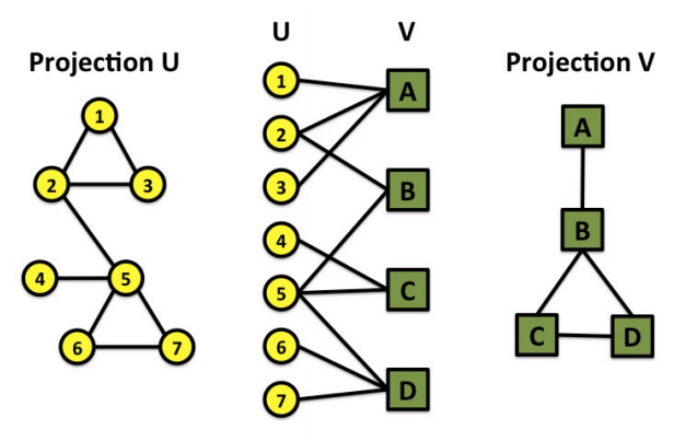
Fig. 193 Folded/projected bipartite graphs
\(r\)-regular graph: A graph \(G\) is \(r\)-regular if \(\operatorname{deg}_G (v)=r\) for all \(v \in V(G)\).
A graph is \(1\)-regular \(\Leftrightarrow\) it is a disjoint union of \(K_2\).
A graph is \(2\)-regular \(\Leftrightarrow\) it is a disjoint union of cycles of any lengths.
\(3\)-regular graph is called cubic. It must have even number of vertices.
A completed graph is \((N_v-1)\)-regular.
Tree and Forest
Definition:
A tree is a connected acyclic graph. Root, leaf, ancestor, descendant, parents, children …
A forest is an acyclic graph.
Characterization: A graph \(G\) is a tree if and only any two of the three conditions hold: connected, acyclic, and \(N_e = N_v - 1\).
Types of trees: star, double star, caterpillar (removing leaves gives the spine)
Claims:
A vertex in a tree is a leaf if it has only one neighbor.
Every tree \(T\) with \(\left\vert V(T) \right\vert \ge\) 2 has at least 2 leaves (two ends of a maximal path).
A connected graph is a tree iff all of its edges are bridges.
Cayley’s Formula: There are \(n^{n-2}\) trees on a vertex set \(V\) of \(n\) elements. Related concept: Prufer Sequence.
Directed acyclic graph: directed and has no cycles.
Note that its underlying undirected graph is not a tree: may contains cycles. Nevertheless, it is often possible to still design efficient computational algorithm on DAGs that take advantage of this near-tree-like structure.
Hamiltonian graph
Hamilton path: a path that covers every vertex once
Hamilton cycle: a cycle that covers every vertex once. A Hamilton cycle can be converted to a Hamilton path by removing one edge.
A graph \(G\) is Hamiltonian if it has a Hamilton cycle.
If \(G\) is Hamiltonian, then any supergraph \(G ^\prime \supseteq G\) where \(G ^\prime\) is obtained by adding new edges between non-adjacent vertices of \(G\), then \(G ^\prime\) is also Hamilton.
A cycle is Hamiltonian.
A complete graph \(K_n\) is Hamiltonian.
A complete bipartite graph \(K_{m,n}\) is Hamiltonian if and only if \(N_v = N_e \ge 2\)
No nice characterization of Hamiltonian graphs.
Planar graph: a graph that can be drawn in the plane, with vertices ad dots and edges as lines, such that no pair of edges intersect.
Heterogeneous graph (node are different kinds of objects)
Multimodal graph (topics, papers, authors, institutions)
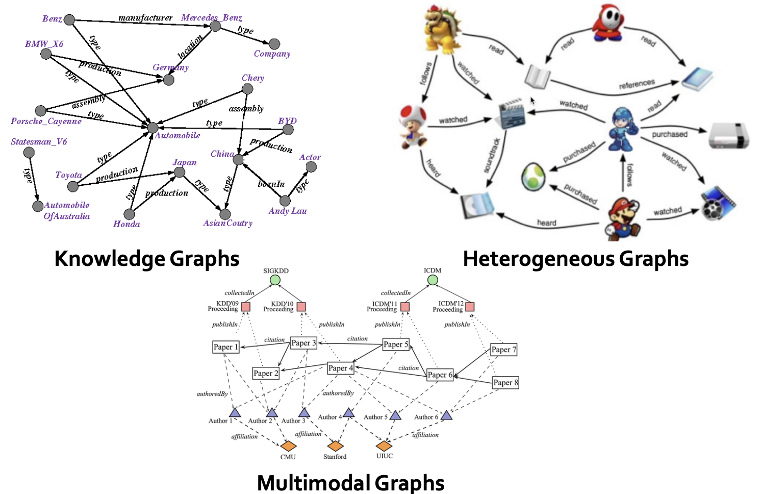
Fig. 194 More types of graphs
Graph-level Concepts
Subgraph: A graph \(F\) is a subgraph of a graph \(G\) if \(V(F)\subseteq V(G)\) and \(E(F)\subseteq E(G)\), also denoted as \(F \subseteq G\).
Spanning subgraph: A spanning subgraph \(F\) is a subgraph obtained only by edge deletions. In other words, \(V(F) = V(G)\) and \(E(F)\subset E(G)\).
Spanning tree: spanning subgraph of \(G\) that is a tree. Every connected graph \(G\) has a spanning tree. Corollary: every connected graph has \(N_e \ge N_v-1\).
Induced subgraph: A induced graph \(F\) is a subgraph obtained only by vertices deletion. If the remaining vertices are \(Y=V(G)\setminus\), we denote \(F\) by \(G[Y]\).
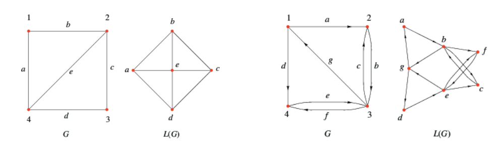
Edge-to-vertex dual graph (line graph): The edge-to-vertex dual graph (line graph) of a directed graph \(G\) is the directed graph \(L(G)\) whose vertex set corresponds to the arc set of \(G\), and having an arc directed from an original edge \(e_1\) to an edge \(e_2\) if in \(G\), the head of \(e_1\) meets the tail of \(e_2\). The line graph for undirected graph can be defined accordingly.
Isomorphic: Two simple graphs \(G\) and \(H\) are isomorphic, denoted \(G \cong H\) if there is a bijection \(\theta: V(G) \rightarrow V(H)\) which preserves adjacency and non-adjacency:
\[ (u,v) \in E(G) \Leftrightarrow (\theta(u), \theta(v)) \in E(H) \]To determine isomorphism of two graphs, we can start by comparing some properties, such as \(N_v\), \(N_e\), \(r\)-regular, number of non-adjacent vertices etc.
Graphlets: graphlets are rooted connected non-isomorphic subgraphs. For a given graph \(G=(V, E)\), non-isomorphic roots node characterizes different graphlets. In the picture below, for 3-node graphs \(G_1, G_2\), \(G_1\) has two non-isomorphic roots, so two graphlets, and \(G_2\) has only 1.
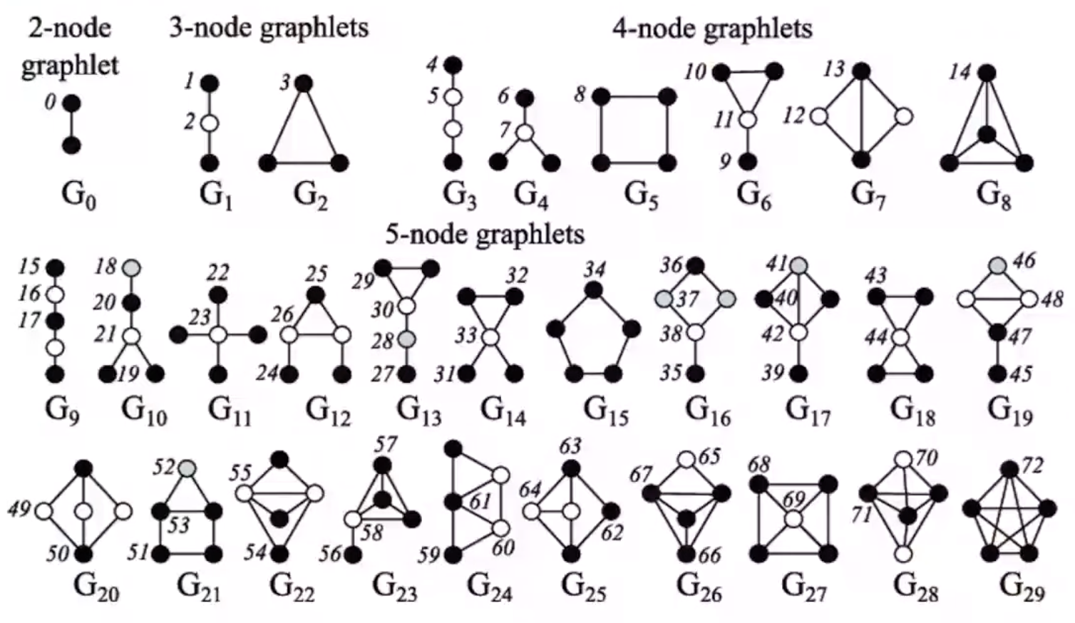
Fig. 196 Graphlets [Przulj et al. 2004]
A decomposition of a graph \(G\) is a family \(\mathcal{F}\) of edge-disjoint subgraphs of \(G\) such that all edges in \(G\) are in some subgraphs.
\[\cup _{F \in \mathcal{F}} E(F) = E(G)\]If every subgraph of \(\mathcal{F}\) is a cycle, then the decomposition is called a cycle decomposition. Similarly, if every subgraph of \(\mathcal{F}\) is a path, then the decomposition is called a path decomposition. A trivial path decomposition exists there each subgraph is an edge. But some graphs have no cycle decomposition.
A graph \(G\) has a cycle decomposition if and only if every vertex in \(G\) has even degree.
Matrices for Graphs
Adjacency Matrix
For an undirected graph \(G\), its adjacency matrix \(\boldsymbol{A}\) is an \(N_v \times N_v\) symmetric binary matrix with entries
Properties
\(\boldsymbol{A} \boldsymbol{1} = \boldsymbol{d}\), i.e. row sum of row \(i\) is the degree of vertex \(i\).
\([\boldsymbol{A} ^r]_{ij}=\) the number of walks of length \(r\) between vertices \(i\) and \(j\)
\(G\) is a regular graph if and only if the maximum degree \(d_{max}\) of \(G\) is an eigenvalue of \(\boldsymbol{A}\).
For directed graphs, its adjacency matrix is defined in a similar way, but it may not be symmetric. Moreover, \(\boldsymbol{A} _{i +} = d_i^{out}\), and \(\boldsymbol{A} _{+j} = d_j^{out}\).
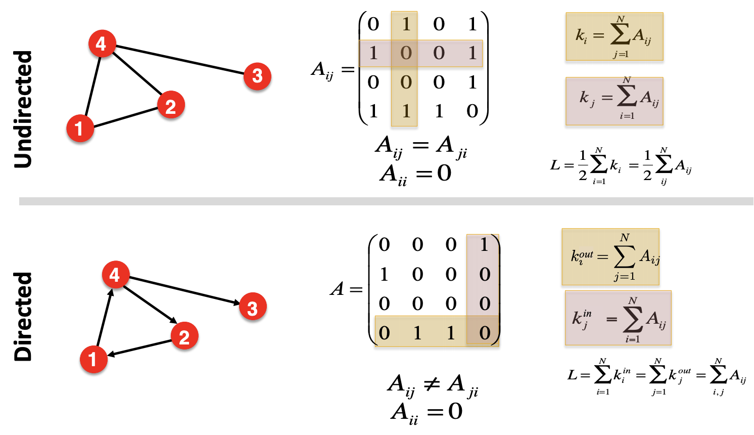
Fig. 197 Adjacency matrix for undirected and directed graph.
Adjacency matrix can also store weights.
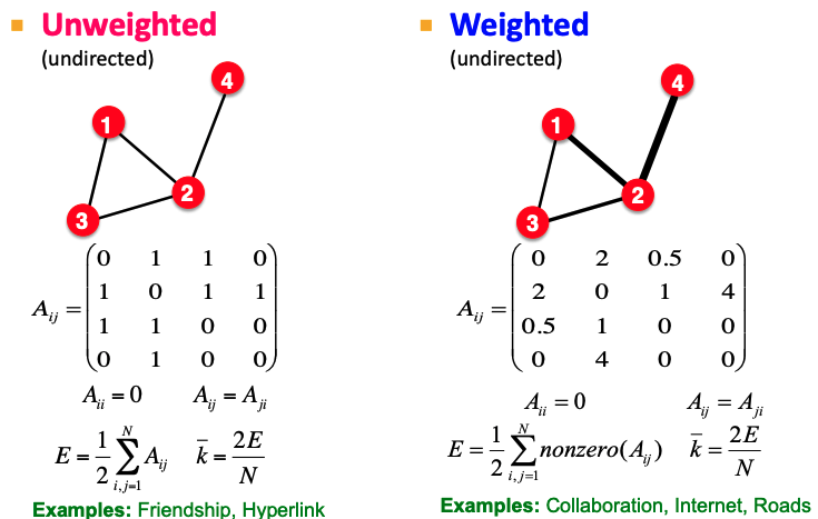
Fig. 198 Adjacency matrix with weights
Laplacian Matrix
Let \(\boldsymbol{D} = \operatorname{diag}\left( \boldsymbol{A} \boldsymbol{1} \right)\) be a diagonal matrix containing the degrees. The laplacian matrix of graph \(G\) is a \(N_v \times N_v\) matrix defined as
It is in analogy to the Laplacian from multivariable calculus (the sum of second partial derivatives of a function), in the sense that
The closer this value is to zero, the more similar are the elements of \(\boldsymbol{x}\) at adjacent vertices in \(V\). Hence, the Laplacian is useful in providing some sense of the ‘smoothness’ of functions on a graph \(G\), with respect to the connectivity of \(G\).
Properties
\(\boldsymbol{L}\) is positive semi-definite, as seen from the above equation
\(\boldsymbol{L} \boldsymbol{1} = \boldsymbol{0}\), i.e. its smallest eigenvalue is 0, with an eigenvector of \(\boldsymbol{1}\). The second smallest eigenvalue is non-trivial, and the arguably most important of all of the eigenvalues, which gives information about its connectivity. In short, the multiplicity of \(0\) equals the number of connected components in \(G\).
Spectra of Laplacian for some common graphs link
The equation above can also be written as
\[ \boldsymbol{x} ^{\top} \boldsymbol{L} \boldsymbol{x} = \frac{1}{2} \sum _{i,j = 1}^n (x_i - x_j)^2 \]where the range of summation changes from \(E\) to \([n] \times [n]\), and there is an additional coefficient \(\frac{1}{2}\).
More definitions of graph Laplacian
If edge weights are given, another way to define the graph Laplacian by replacing \(\boldsymbol{A}\) by \(\boldsymbol{W}\) is defined as:
\[ \boldsymbol{L} _W = \boldsymbol{D} _W - \boldsymbol{W} \]where \(\boldsymbol{D} _W = \boldsymbol{W} \boldsymbol{1}\). The corresponding equation becomes
\[ \boldsymbol{x} ^{\top} \boldsymbol{L} _W \boldsymbol{x} = \frac{1}{2} \sum _{i,j = 1}^n w_{ij} (x_i - x_j)^2 \]To prove it (and the equations above), use
\[\begin{split} \begin{aligned} \sum_{i, j} w_{i j}\left(x_{i}-x_{j}\right)^{2} &=\sum_{i, j} w_{i j} x_{i}^{2}+\sum_{i, j} w_{i j} x_{j}^{2}-2 \sum_{i, j} w_{i j} x_{i} x_{j} \\ &=\sum_{i} d_{W, i} x_{i}^{2}+\sum_{j} d_{W, j} x_{j}^{2}-2 \sum_{i, j} w_{i j} x_{i} x_{j} \\ &=2 \boldsymbol{x}^{\top} \boldsymbol{D}_W \boldsymbol{x} -2 \boldsymbol{x}^{\top} \boldsymbol{W} \boldsymbol{x} \\ &=2 \boldsymbol{x}^{\top}(\boldsymbol{D}_W-\boldsymbol{W}) \boldsymbol{x} \\ &=2 \boldsymbol{x}^{\top} \boldsymbol{L}_W \boldsymbol{x} . \end{aligned} \end{split}\]The symmetric normalized Laplacian is defined as
\[\begin{split}\begin{aligned} \boldsymbol{L} ^\mathrm{sym} &= \boldsymbol{D} ^{-1/2} \boldsymbol{L} \boldsymbol{D} ^{-1/2} \\ &= \boldsymbol{I} - \boldsymbol{D} ^{-1/2} \boldsymbol{A} \boldsymbol{D} ^{-1/2} \\ [\boldsymbol{L} ^\mathrm{sym}]_{ij}&= \left\{\begin{array}{ll} 1 & \text { diagonal and } \operatorname{deg}\left(v_{i}\right) \neq 0 \\ -\frac{1}{\sqrt{\operatorname{deg}\left(v_{i}\right) \operatorname{deg}\left(v_{j}\right)}} & \text { off-diagonal and } (i, j) \in E\\ 0 & \text { otherwise. } \end{array}\right.\\ \end{aligned}\end{split}\]The matrix \(\boldsymbol{I} - \boldsymbol{L} ^{\mathrm{sym}}\) is similar to \(\boldsymbol{D} ^{-1} \boldsymbol{A}\):
\[ \boldsymbol{D} ^{-1} \boldsymbol{A} = \boldsymbol{D} ^{-1/2} (\boldsymbol{I} - \boldsymbol{L} ^{\mathrm{sym}}) \boldsymbol{D} ^{1/2} \]The random-walk normalized Laplacian matrix is defined as
\[\begin{split}\begin{aligned} \boldsymbol{L} ^\mathrm{rw} &= \boldsymbol{D} ^{-1} \boldsymbol{L} \\ &= \boldsymbol{I} - \boldsymbol{D} ^{-1} \boldsymbol{A} \\ [\boldsymbol{L} ^\mathrm{rw}]_{ij}&= \left\{\begin{array}{ll} 1 & \text { if } i=j \text { and } \operatorname{deg}\left(v_{i}\right) \neq 0 \\ -\frac{1}{\operatorname{deg}\left(v_{i}\right)} & \text { if } i \neq j \text { and } v_{i} \text { is adjacent to } v_{j} \\ 0 & \text { otherwise. } \end{array}\right.\\ \end{aligned}\end{split}\]As its name suggests, it is related to random walk. The matrix \(\boldsymbol{D} ^{-1} \boldsymbol{A} = \boldsymbol{I} - \boldsymbol{L} ^{\mathrm{rw}}\) is row stochastic: every row sum = 1, which can be used as an transition matrix \(\boldsymbol{P}\). Precisely,
\[\begin{split} p_{ij} = \left\{\begin{array}{ll} 1/d_i, & \text { if } (i,j) \in E \\ 0, & \text { otherwise } \end{array}\right. \end{split}\]\(L^\mathrm{rw}\) and \(L^\mathrm{sym}\) are similar:
\[ \underbrace{\boldsymbol{D}^{-1} \boldsymbol{L}}_{\boldsymbol{L}^{\mathrm{rw}}}=\underbrace{\boldsymbol{D}^{-1 / 2}}_{\boldsymbol{P}^{-1}} \underbrace{\boldsymbol{D}^{-1 / 2} \boldsymbol{L} \boldsymbol{D}^{-1 / 2}}_{\boldsymbol{L}^{\mathrm{sym}}} \underbrace{\boldsymbol{D}^{1 / 2}}_{\boldsymbol{P} } \]which implies that
both matrices have the same eigenvalues
\[ 0=\lambda_{1} \leq \lambda_{2} \leq \cdots \leq \lambda_{n} \]Additionally, it can be shown that the multiplicity of the zero eigenvalue is also equal to the number of connected components in the graph.
a vector \(\boldsymbol{v}\) is an eigenvector of \(\boldsymbol{L} ^\mathrm{rw}\) if and only if the vector \(\boldsymbol{D} ^{1/2}\boldsymbol{v}\) is an eigenvector of \(\boldsymbol{L} ^\mathrm{sym}\).
\[ \underbrace{\boldsymbol{D}^{-1} \boldsymbol{L}}_{\boldsymbol{L}_{\mathrm{rw}}} \boldsymbol{v}=\lambda \boldsymbol{v} \Longleftrightarrow \underbrace{\boldsymbol{D}^{-1 / 2} \boldsymbol{L} \boldsymbol{D}^{-1 / 2}}_{\boldsymbol{L}^{\mathrm{sym}}} (\boldsymbol{D}^{1 / 2} \boldsymbol{v})=\lambda (\boldsymbol{D}^{1 / 2} \boldsymbol{v} ) \]In particular, for the eigenvalue 0, the associated eigenvectors for \(\boldsymbol{L}^\mathrm{rw}\) and \(\boldsymbol{L} ^\mathrm{sym}\) are \(\boldsymbol{v} _1 = \boldsymbol{1}\) and \(\boldsymbol{u} _1 = \boldsymbol{D} ^{1/2}\boldsymbol{1}\) respectively. Also note that \(0 = \boldsymbol{u} _2 ^{\top} \boldsymbol{u} _1 = \boldsymbol{v} _2 ^{\top} \boldsymbol{D} \boldsymbol{v} _1 = \boldsymbol{v} _2 ^{\top} \boldsymbol{D} \boldsymbol{1}\).
The additive normalized Laplacian is defined as
\[ \boldsymbol{L} ^{\mathrm{add}} = \frac{1}{d_\max} (\boldsymbol{A} + d_\max \boldsymbol{I} - \boldsymbol{D} ) = \frac{1}{d_\max}(d_\max \boldsymbol{I} - \boldsymbol{L} ) \]It has same eigenvectors with \(\boldsymbol{L}\) but different eigenvalues
\[ \boldsymbol{L}^{\mathrm{add}} \boldsymbol{u}=\beta \boldsymbol{u} \Longleftrightarrow \boldsymbol{L} \boldsymbol{u}=\lambda \boldsymbol{u}\qquad \beta=1-\frac{\lambda}{d_{\max }} \]The weighted analogies for \(\boldsymbol{L} ^\mathrm{sym}, \boldsymbol{L} ^\mathrm{rw}, \boldsymbol{L} ^{\mathrm{add}}\) are defined accordingly.
Incidence Matrix
The incidence matrix \(\boldsymbol{B}\) of a graph \(G\) is an \(N_v \times N_e\) binary matrix with entries
Properties
If we extend \(\boldsymbol{B}\) to a signed incidence matrix \(\tilde{\boldsymbol{B}}\), by arbitrarily assigning direction to all edges, and let \(\tilde{b}_{ij}=1\) and \(\tilde{b}_{ji}=-1\) if \((i,j)\) is a directed edge, then we can show that
\[ \tilde{\boldsymbol{B} }\tilde{\boldsymbol{B} }^{\top} = \boldsymbol{L} \]\(\texttt{RowSum}(v)= \operatorname{deg} (v)\) and \(\texttt{ColSum} = 2\).
If there exists self-loop \(j\) of vertex \(i\), then \(M_{ij}=2\).
Routing matrix
Suppose there \(N_v \times N_v\) pairwise traffic flows between each pair of vertices. A routing matrix \(\boldsymbol{R}\) is a \(N_e \times N_v^2\) binary matrix,
Data Structure to Represent a Graph
The most intuitional representation is by an \(N_v \times N_v\) adjacency matrix defined previously. It contains binary entries, which is \(1\) if there is an edge between vertices \(i\) and \(j\), and zero otherwise. The memory required is \(O(N_v^2)\).
Most real-world networks are sparse, in the sense that \(N_e \sim N_v\), or \(\bar{d} \ll N_v-1\), so the adjacency matrix is sparse. It is preferable to use adjacency list. But the simplicity of the adjacency matrix representation may sometimes be felt to outweigh any memory disadvantages, especially for smaller graphs.
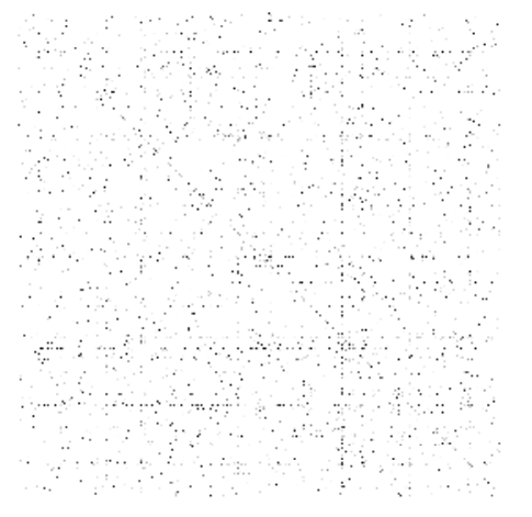
Fig. 199 Sparse adjacency matrix
Other data structures include
Edge List
\(N_e\) objects in the two-column list, each object represents an edge, and stores the pair of vertices of that edge. Memory \(O(m)\)
Adjacency List
\(N_v\) objects in the list, each object represents a vertex, and stores a list of neighbors of that vertex.
Easy to work with large and sparse graphs
Allows us to quickly retrieve all neighbors of a given vertex
Memory \(O(n + m)\)
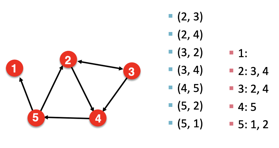
Fig. 200 Edge list and adjacency list
Incidence matrix
\(O(nm)\)
Algorithms
BFS
Core of Prim’s, Dijkstra’s
DFS
sub-routine of topological sort, which can be used to determine whether a directed graph \(G\) is acyclic, and algorithms for decomposing \(G\) into its strongly connected components.
finding a maximal clique is NP-hard
Exercise
Prove or disapprove: For three vertices \(u, v, w \in V(G)\), if there is an even-length path from \(u\) to \(v\) and an even-length path from \(v\) to \(w\), then there is an even-length path from \(u\) to \(w\).
Solution
False.
\[\begin{split}\begin{aligned} &\ v \\ &/ \ \backslash \\ u-w&-\circ \\ \end{aligned}\end{split}\]Every vertex in \(G\) has even degree, if only if
\(G\) has a cycle decomposition
\(G\) has an Euler tour.
Theorems
If in a graph \(G\), all vertices have degree at least 2, then \(G\) contains a cycle.
A graph \(G\) is bipartite \(\Leftrightarrow\) it contains no odd cycle.
An edge \(e \in E(G)\) is a bridge \(\Leftrightarrow\) \(e\) is not in any cycle of \(G\) (proof by contrapositive).
A graph \(G\) is a tree \(\Leftrightarrow\) \(G\) is acyclic and \(N_e = N_v -1\).
A connected graph is a tree iff all of its edges are bridges.
A \(k\)-coloring of graph \(G\) partitions the vertex set \(V\) into \(k\) independent sets \(V_1, \ldots, V_k\).