Variational Autoencoders
More or less simultaneously proposed by Kingma & Welling (2013) and Rezende et al. (2014). A good introduction is done by Dürr (2016). Besides, Zhao et el. (2017) made a paper for deeper understanding.
VAE is a type of generative model for a vector of random variables \(\boldsymbol{x}\) assumed to be generated from a set of latent variables \(\boldsymbol{z}\). Assuming both \(\boldsymbol{x} \in \mathbb{R}^D\) and \(\boldsymbol{z} \in \mathbb{R}^J\) are continuous, the unconditional distribution of \(\boldsymbol{x}\) can be written as
Initially used for generation, VAE has also been successful for representation learning. It is popular, fast, and relatively easy to train.
VAE have similar structure with AE. But we add probabilistic assumptions of the VAE representation and optimize the VAE objective via variational optimization.
Objective
Ideally, the encoder and decoder should learn the two conditional distributions (from the joint distribution of \((x,z)\)) parameterized by \(\theta\).
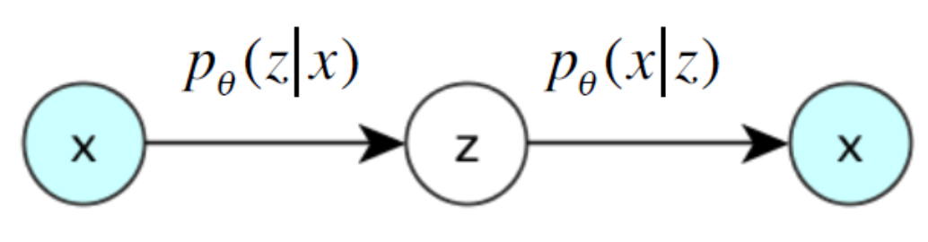
Fig. 167 Ideal case of VAE [Durr 2016]
But \(p(\boldsymbol{z} \vert \boldsymbol{x} )\) can be very costly to estimate. As a result, we approximate it with another neural function \(q(\boldsymbol{z} \vert \boldsymbol{x} )\), which is the decoder.
Assume w.l.o.g. that latent variable \(\boldsymbol{z}\) is 1-dimensional, \(\boldsymbol{x}\) is 2-dimensional. The VAE structure can be shown as
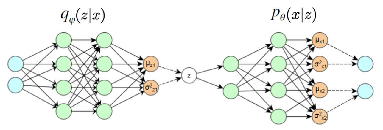
Fig. 168 VAE structure (dash lines mean sampling) [Durr 2016]
\(q(\boldsymbol{x} \vert \boldsymbol{z} )\) is the distribution learned by the encoder part.
\(p(\boldsymbol{x} \vert \boldsymbol{z})\) is the distribution learned by the decoder part.
The orange nodes in the middle and at the right are the parameters in the distribution \(q(\boldsymbol{z})\) and \(p(\boldsymbol{x})\) respectively.
After the model is trained, we have
a learned representation described by \(q(\boldsymbol{z})\). To output a single value, we can use the mean, or mode.
a generator \(p(\boldsymbol{x} \vert \boldsymbol{z} )\). To generate \(\boldsymbol{x}\) (e.g. an image) given \(\boldsymbol{z}\), we can use the decoder network.
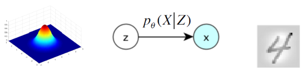
Fig. 169 Use VAE to generate a handwritten digit [Durr 2016]
There is a theoretical foundation of generation.
- Theorem (Validation of VAE)
Any \(d\)-dimensional distribution can be generated by taking \(d\) normally distributed variables and mapping them through some appropriate (possibly very complicated) function.
Of course, the function can be a neural network.
Training
Variational Optimization
Directly Maximizing the likelihood can be challenging. Instead, we maximize the lower bound of the likelihood.
By some formula from conditional probability and information theory, we have
If we can well approximate \(p(z \vert x)\) by \(q(z \vert x)\), then the KL divergence is small, and we can maximizing \(L\) by maximizing \(L^v\).
The lower bound \(L^v\) can be further arranged to
We then maximizing the last line.
The first term is the negative KL divergence between the posterior and the prior (often Gaussian). We want to minimize the distance. It can be viewed as a regularizer.
When \(p(z) = \mathcal{N} (0, 1)\) and \(q(z|x)\) is also Gaussian, this KL divergence has a closed form
\[ -\operatorname{KL} \left[ q\left(z \vert x_{i}\right), p(z) \right]=\frac{1}{2} \sum_{j=1}^{J} 1+\log \left(\sigma_{z_{i, j}}^{2}\right)-\mu_{z_{i, j}}^{2}-\sigma_{z_{i, j}}^{2} \]where \(J\) is the dimension of \(\boldsymbol{z}\). See the previous VAE structure plot where \(J=1\).
The second term can be seen as a reconstruction loss, which equals \(\log(1)\) if \(\boldsymbol{x}_i\) is perfectly reconstructed from \(\boldsymbol{z}\). In training, the expectation is estimated by sampling \(B\) samples \(z_{j,l}\) from the encoder network \(q(z\vert x_i)\) and compute the average of \(\log p\left(x_{i} \mid z_{i, l}\right)\)
\[ \mathbb{E}_{q(z \vert x)}\left[ \log p(x \vert z) \right] = \frac{1}{B} \sum_{l=1}^{B}\log p\left(x_{i} \vert z_{i, l}\right) \]If \(p(x \vert z)\) is Gaussian and \(B=1\) (often used), then it is just a least squares loss
\[ \log p\left(x_{i} \vert z_{i}\right)=\sum_{j=1}^{D} \frac{1}{2} \log \sigma_{x_{j}}^{2}+\frac{\left(x_{i, j}-\mu_{x_{j}}\right)^{2}}{2 \sigma_{x_{j}}^{2}} \]where \(D\) is the dimension of \(\boldsymbol{x}\).
Hence, the overall objective of VAE is: We want the representation \(\boldsymbol{x}\) be as accurate as possible (KL divergence), and use it to reconstruct \(\boldsymbol{x}\) as accurate possible (reconstruction loss).
In practice, we can add a hyperparamter: weight coefficient, to one of the two terms.
VAE vs denoising AE
Denoising AE:
\[ \boldsymbol{x} + \boldsymbol{\varepsilon} \overset{\text{encoder}}{\longrightarrow} \boldsymbol{z} \overset{\text{decoder}}{\longrightarrow} \boldsymbol{x} ^\prime \]with reconstruction loss \(\left\| \boldsymbol{x} - \boldsymbol{x} ^\prime \right\|^2\).
VAE:
\[\begin{split} \left.\begin{array}{ll} \boldsymbol{x} \overset{\text{encoder}}{\longrightarrow} &\boldsymbol{z} \\ &+\\ &\boldsymbol{\varepsilon} \end{array}\right\} \overset{\text{decoder}}{\longrightarrow} \boldsymbol{x} ^\prime \end{split}\]with reconstruction loss \(\left\| \boldsymbol{x} - \boldsymbol{x} ^\prime \right\|^2\) and a KL divergence regularizer between prior \(p(\boldsymbol{z})\) and posterior \(q(\boldsymbol{z} \vert \boldsymbol{x})\).
Reparameterization Trick
Note that at the end of the encoder part, we have the neurons that corresponds to the parameters in \(q(\boldsymbol{z})\), then we sample \(\boldsymbol{z}\). Then \(z\) is random in the back. The question is, how to do backpropagation through this random node?
A trick is to reparameterize \(\boldsymbol{z}\) by
where \(\boldsymbol{\varepsilon} \sim N(\boldsymbol{0}, \boldsymbol{I})\) can be viewed as noise.
Then random node becomes \(\boldsymbol{\varepsilon}\), and we won’t need to compute its gradient during backpropagation.
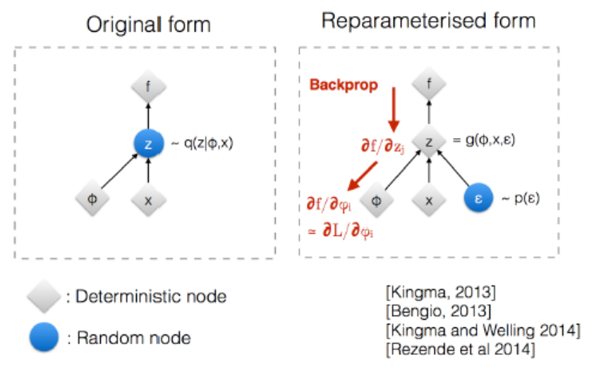
Fig. 170 Reparametrization trick of VAE [Kingma 2015]
Interpretation
By Phase Diagrams
After obtaining \(q(\boldsymbol{z})\), we can create a phase diagram with varying values in each dimension \(z_1, z_2, \ldots, z_k\), and then pass them to decoder to generate \(\boldsymbol{x}\), then we can see that how these \(\boldsymbol{z}\)’s differ according to varying values of \(z_1, z_2, \ldots, z_k\), and the difference along dimension \(j\) can be interpreted as the learned representation by \(z_j\).
In the following example (a), \(k=2\), the horizontal dimension is head tile, and the vertical dimension is degree of smiling vs frowning.
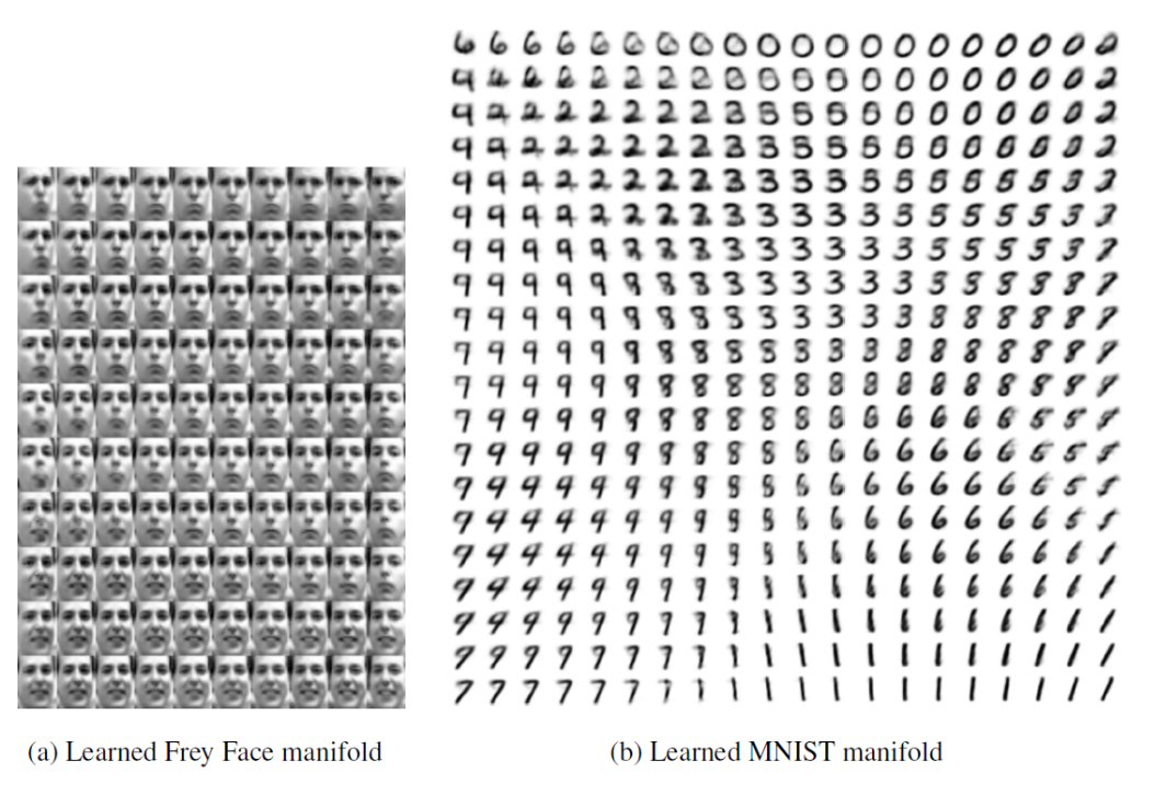
Fig. 171 VAE phase diagram for interpretation
Potential Representations
Interpretable dimensions of continuous variation can be
Images: facial expression, digit writing style, …
Music: pitch, timbre, …
Speech audio: speaker characteristics, emotion, …
Text: shades of meaning, sentiment, ..
Interpretable dimensions of discrete variation dimensions can be
Images: digit identity, face identity, object type, …
Music: instrument identity, discrete pitch, …
Speech audio: phoneme, word, language, …
Text: part of speech, phrase (constituent) type, topic, …
Or, the representation just learn signal and get rid of noise.
Generation
Option 1. Draw \(\boldsymbol{z}\) from the prior \(p(\boldsymbol{z})\), feed through decoder to generate \(\hat{\boldsymbol{x}}\). [Details]
Option 2: Generation based on one or more examples \(\boldsymbol{x}\)
Draw \(\boldsymbol{z}\) from \(q(\boldsymbol{z} |\boldsymbol{x})\)
Optionally, adjust \(\boldsymbol{z}\) (e.g. interpolate \(\boldsymbol{z} _1, \boldsymbol{z} _2\) between multiple samples \(\boldsymbol{x}_1, \boldsymbol{x} _2\))
Feed through the decoder to generate more examples \(\hat{\boldsymbol{x}}\)
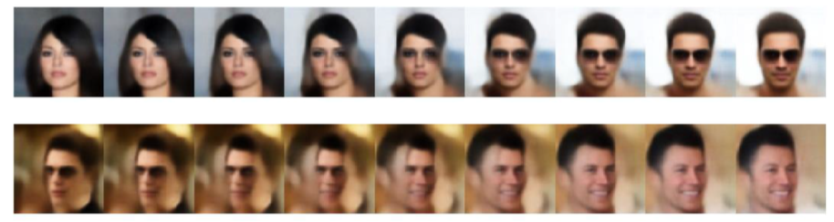
Fig. 172 VAE for generation
Compared to autoregressive models:
In autoregressive models, e.g. RNN or PixelRNN, we need to define the order/dependency of generated text/pixels. While in VAE, all outputs are generated jointly from the latent variables \(\boldsymbol{z}\), so it can model arbitrary dependencies.
More flexible: Can tweak \(\boldsymbol{z}\) to control generation
Usually, more efficient to sample from distribution
Tend to produce blurrier outputs, since we are sampling from distribution and look at mean (averaging the details)
Extension
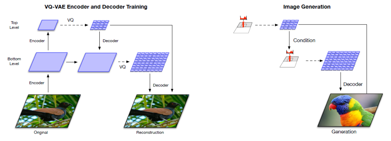
VQ-VAE
[van den Oord et al. 2018]
VQ-VAE is a kind of discrete representation learning. There is a clustering step (vector quantization) layer in VAE. In images, some discrete representations can be, for instance, edge, border, or eye, nose, ear …
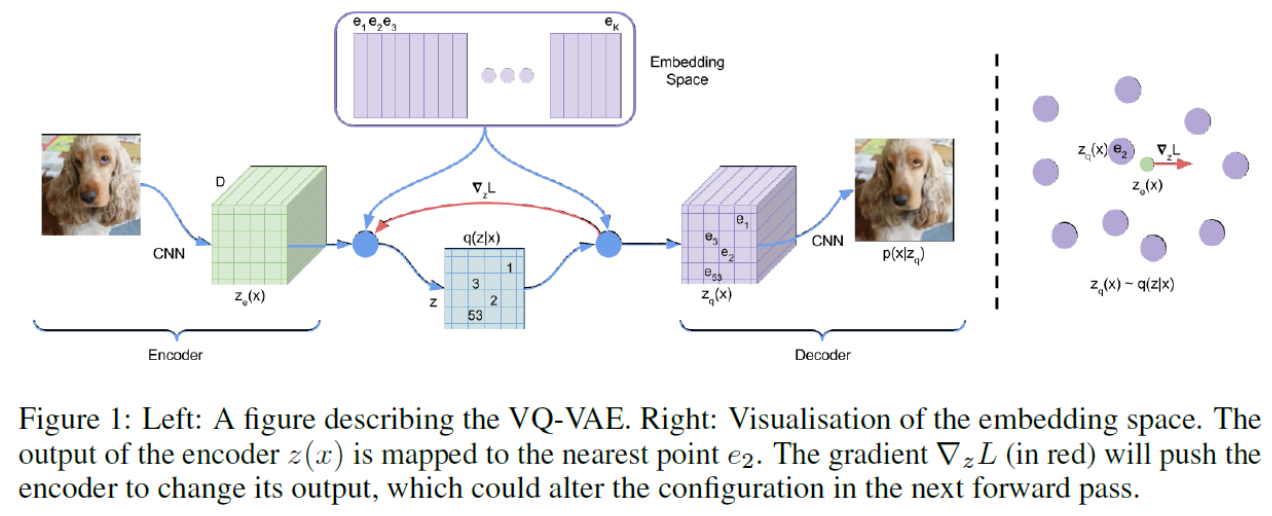
Fig. 173 Illustration of VQ-VAE
The loss is
where
KL divergence in VAE becomes constant
Reconstruction error becomes squared error between \(z_e(x)\) and embedding \(e\).
In backpropagation, skip discretization layers.