Theory
We introduced some theory behind classification for two populations \(\pi_1, \pi_2\), as well as generalization to \(g\) populations \(\pi_j, j=1, 2, \ldots, g\).
Setup
Regions
For a classifier with some classification rule, let
\(\Omega\) be the sample space of all possible values of \(\boldsymbol{x}\)
\(R_1\) be the set (or region) of all \(\boldsymbol{x}\) values for which we classify objects as \(\pi_1\) by this rule
\(R_2 = \Omega \setminus R_1\) be the remaining \(\boldsymbol{x}\)
PDF
In theory, let \(f_i(\boldsymbol{x})\) be the probability density function for \(i\)-th population, \(i=1,2\). We can then define \(\mathbb{P} (i \vert j)\) be the probability of classifying \(\boldsymbol{x}\) in \(\pi_i\) by the rule, given that in fact \(\boldsymbol{x}\) is from \(\pi_j\). Then
Priors
Suppose the prior probability of a random sampled observation belonging to \(\pi_i\) is
\[
\mathbb{P} (\pi_i) = \pi _i
\]
with \(\sum_{i=1} p_i = 1\). Then we have
\(\mathbb{P}(i \vert i) p_i\) is the probability that a randomly sampled observation correctly classified as \(\pi_i\)
\(\sum_{j\ne i}\mathbb{P}(i \vert j) p_j\) is the probability that a randomly sampled observation incorrectly classified as \(\pi_i\)
Cost
Usually, there is cost of misclassification. Let \(c(i \vert j)\) be the cost of wrongly classifying an object from class \(j\) to class \(i\). Note that
Global Measurements and Learning
Based on the quantity above, we can then define some global measurement of classification. Then we can choose \(R_1, R_2\) to minimize them.
Expected Cost of Misclassification
The expected cost of misclassification (ECM) is defined as
\[\begin{split}\begin{aligned}
\text{ECM}
&=\mathbb{E} \left(\text{cost of misclassifying the object into $\pi_{2} \vert$ an object is from } \pi_{1}\right) p_{1} \\
&+\mathbb{E} \left(\text{cost of misclassifying the object into $\pi_{1} \vert$ an object is from } \pi_{2}\right) p_{2} \\
&=c(2 \vert 1) \mathbb{P} (2 \vert 1) p_{1}+c(1 \vert 2) \mathbb{P} (1 \vert 2) p_{2}\\
\end{aligned}\end{split}\]
To find an optimal classifier, the region \(R_1, R_2\) can be optimized to minimize the ECM. It can be shown that the optimal \(R_1\), \(R_2\) is
\[\begin{split}
\begin{array}{l}
R_{1}^{\text{ECM} }=\left\{x: \frac{f_{1}(x)}{f_{2}(x)} \geq \frac{c(1 \vert 2)}{c(2 \vert 1)} \cdot \frac{p_{2}}{p_{1}}\right\} \quad\left(\begin{array}{c}
\text { density } \\
\text { ratio }
\end{array}\right) \geq\left(\begin{array}{c}
\text { cost } \\
\text { ratio }
\end{array}\right)\left(\begin{array}{l}
\text { prior } \\
\text { ratio }
\end{array}\right) \\
R_{2}^{\text{ECM} }=\left\{x: \frac{f_{1}(x)}{f_{2}(x)}<\frac{c(1 \vert 2)}{c(2 \vert 1)} \cdot \frac{p_{2}}{p_{1}}\right\} \quad\left(\begin{array}{c}
\text { density } \\
\text { ratio }
\end{array}\right)<\left(\begin{array}{c}
\text { cost } \\
\text { ratio }
\end{array}\right)\left(\begin{array}{l}
\text { prior } \\
\text { ratio }
\end{array}\right)
\end{array}
\end{split}\]
Proof
Substituting the definition of \(\mathbb{P} (i\vert j)\) we have
\[\begin{split}
\begin{aligned}
\text{ECM} &=p_{1} c(2 \vert 1) \int_{\Omega \backslash R_{1}} f_{1}(x) d x+p_{2} c(1 \vert 2) \int_{R_{1}} f_{2}(x) d x \\
&=p_{1} c(2 \vert 1) \int_{\Omega} f_{1}(x) d x-p_{1} c(2 \vert 1) \int_{R_{1}} f_{1}(x) d x+p_{2} c(1 \vert 2) \int_{R_{1}} f_{2}(x) d x \\
&=p_{1} c(2 \vert 1)+\int_{R_{1}}\left[p_{2} c(1 \vert 2) f_{2}(x)-p_{1} c(2 \vert 1) f_{1}(x)\right] d x
\end{aligned}
\end{split}\]
The first term \(p_1 c(2 \vert 1) \ge 0\) is a constant. To minimize ECM is to minimize the second term. Hence, \(R_1\) only covers the region of \(x\) where \(p_{2} c(1 \vert 2) f_{2}(x)-p_{1} c(2 \vert 1) f_{1}(x) < 0\). That is,
\[
R_1 = \left\{ x: \frac{f_{1}(x)}{f_{2}(x)} \geq \frac{c(1 \vert 2)}{c(2 \vert 1)} \cdot \frac{p_{2}}{p_{1}}\right\}
\]
For multiple classes,
the expected cost of misclassifying an item \(x\) from \(\pi_i\) is
\[\text{ECM}(i) = \sum_{j=1}^g c(j \vert i) \mathbb{P} (j \vert i)\]
with \(c(i \vert i) = 0\).
the expected cost over all items is
\[\text{ECM} = \sum_{j=1}^g p_i \text{ECM}(i)\]
The classification regions \(R_k, k = 1, 2, \ldots, g\) that minimize the overall expected cost of misclassification ECM are defined by allocating observation \(x\) to population \(\pi_k\) for which the misclassification cost is minimized.
\[
R_{k}=\left\{x: \sum_{i=1, i \neq k}^{g} p_{i} f_{i}(x) c(k \vert i) \leq \sum_{i=1, i \neq \ell}^{g} p_{i} f_{i}(x) c(\ell \vert i), \quad \ell=1, \cdots, g \right\}
\]
If costs are even then this becomes
\[
R_{k}=\left\{x: p_{k} f_{k}(x) \geq p_{i} f_{i}(x), \forall\ i \ne k\right\}
\]
Total Probability of Misclassification
Another global measurement is total probability of misclassification (TPM), defined as
\[
\text{TPM} =p_{1} \int_{R_{2}} f_{1}(x) d x+p_{2} \int_{R_{1}} f_{2}(x) d x
\]
Minimizing TPM is the same as minimizing ECM when misclassification costs \(c(j \vert i), j \ne i\) are the same for all classes. The regions are simplified to
\[\begin{split}
\begin{array}{l}
R_{1} ^{\text{TPM} }=\left\{x: \frac{f_{1}(x)}{f_{2}(x)} \geq \frac{p_{2}}{p_{1}}\right\} \quad\left(\begin{array}{c}
\text { density } \\
\text { ratio }
\end{array}\right) \geq\left(\begin{array}{l}
\text { prior } \\
\text { ratio }
\end{array}\right) \\
R_{2}^{\text{TPM} }=\left\{x: \frac{f_{1}(x)}{f_{2}(x)}<\frac{p_{2}}{p_{1}}\right\} \quad\left(\begin{array}{c}
\text { density } \\
\text { ratio }
\end{array}\right)<\left(\begin{array}{l}
\text { prior } \\
\text { ratio }
\end{array}\right)
\end{array}
\end{split}\]
Bayesian Approach
Bayesian approach allocate a new observation \(x_0\) to the class with largest posterior probability \(\mathbb{P} (\pi_i \vert x_0)\). By Bayes’ Rule, the posterior probability is
\[\begin{split}
\begin{aligned}
\mathbb{P}(\pi_{1} \vert x_{0}) &=\frac{\mathbb{P}(\text {we observe } x_{0}, \text { and } x_{0} \text { is from } \pi_{1})}{\mathbb{P}(\text {we observe } x_{0})} \\
&=\frac{\mathbb{P}(\text {we observe } x_{0} \vert \pi_{1}) \mathbb{P}(\pi_{1})}{\mathbb{P}(\text {we observe } x_{0} \vert \pi_{1}) \mathbb{P}(\pi_{1})+\mathbb{P}(\text {we observe } x_{0} \vert \pi_{2}) \mathbb{P}(\pi_{2})} \\
&=\frac{f_{1}(x_{0})p_{1} }{f_{1}(x_{0})p_{1}+ f_{2}(x_{0})p_2}
\end{aligned}
\end{split}\]
Hence, the Bayesian classifier assign \(x_0\) to \(\pi_1\) if \(\mathbb{P}\left(\pi_{1} \vert x_{0}\right) \ge \mathbb{P}\left(\pi_{2} \vert x_{0}\right)\), which is
\[
R_{1}^{\text{Bay} }=\left\{x: \frac{f_{1}(x)}{f_{2}(x)} \geq \frac{p_{2}}{p_{1}}\right\}
\]
We conclude that
In terms of classification regions, maximizing posterior probability is equivalent to minimizing the Total Probability of Misclassification TPM.
However the values of the posterior probability \(\mathbb{P}\left(\pi_{1} \vert x_{0}\right)\) provide more information than the yes-or-no class boundaries, especially in the not so clear-cut cases.
For multi-classes, the posterior probability that \(x_0\) is from \(\pi_k\) is
\[
\mathbb{P} \left(\pi_{i} \mid x_{0}\right)=\frac{p_{i} f_{i}\left(x_{0}\right)}{\sum_{j=1}^{g} p_{j} f_{j}\left(x_{0}\right)}=\frac{p_{i} f_{i}\left(x_{0}\right)}{p_{1} f_{1}\left(x_{0}\right)+\cdots+p_{g} f_{g}\left(x_{0}\right)}
\]
In applications, the quantities \(p_i\) and \(f_i\) are often not known given data. Estimation procedures have to be developed to apply these criteria. For instance,
Errors
Optimum error rate, aka minimum total probability of misclassification
\[\begin{split}\begin{aligned}
\text{OER}
&= \min_{R_1, R_2} \text{TPM} \\
&= \min_{R_1, R_2} p_{1} \int_{R_{2}} f_{1}(\boldsymbol{x}) d x+p_{2} \int_{R_{1}} f_{2}(x) d x
\end{aligned}\end{split}\]
Under equal cost, we have
\[\text{OER} = \min_{R_1, R_2} \text{TPM} = \min_{R_1, R_2} \text{ECM}\]
Actual error rate
\[
\text{AER} =p_{1} \int_{\hat{R}_{2}} f_{1}(\boldsymbol{x}) d x+p_{2} \int_{\hat{R}_{1}} f_{2}(x) d x
\]
\(\hat{R}\) are regions learned from data by some rule.
\(f(x)\) are still unknown, hence AER cannot be calculated
Apparent error rate, aka training error rate, which is the fraction of
observations in the training sample that are misclassified.
\[
\text{APER} = \frac{\# \left\{ \text{misclassified} \right\}}{N} = 1 - \text{accuracy}
\]
We can train a classifier in training set, and compute APER in test set. It can then be used as an approximation for \(\mathbb{E} [AER]\).
Equal Covariance
Two-classes
Let the populations \(\pi_i, i=1,2\) be multivariate Gaussian with density \(\mathcal{N} _p (\boldsymbol{\mu} _i, \boldsymbol{\Sigma})\). The classification rule that minimizes ECM is to allocate \(\color{teal}{\boldsymbol{x}_{0}}\) to \(\pi_1\) if
\[
\left(\boldsymbol{\mu}_{1}-\boldsymbol{\mu}_{2}\right)^{\top} \boldsymbol{\Sigma} ^{-1} {\color{teal}{\boldsymbol{x}_{0}}} -\frac{1}{2}\left(\boldsymbol{\mu}_{1}-\boldsymbol{\mu}_{2}\right)^{\top} \boldsymbol{\Sigma} ^{-1}\left(\boldsymbol{\mu}_{1}+\boldsymbol{\mu}_{2}\right) \geq \ln \left(\frac{c(1 \vert 2)}{c(2 \vert 1)} \cdot \frac{p_{2}}{p_{1}}\right)
\]
Proof
Since
\[\begin{split}\begin{aligned}
\log\frac{f_{1}(\boldsymbol{x})}{f_{2}(\boldsymbol{x})}
&=-\frac{1}{2}\left[\left(\boldsymbol{x}-\boldsymbol{\mu}_{1}\right)^{\top} \boldsymbol{\Sigma}^{-1}\left(\boldsymbol{x}-\boldsymbol{\mu}_{1}\right)-\left(\boldsymbol{x}-\boldsymbol{\mu}_{2}\right)^{\top} \boldsymbol{\Sigma}^{-1}\left(\boldsymbol{x}-\boldsymbol{\mu}_{2}\right)\right] \\
&=\left(\boldsymbol{\mu}_{1}-\boldsymbol{\mu}_{2}\right)^{\top} \boldsymbol{\Sigma}^{-1} \boldsymbol{x}-\frac{1}{2}\left(\boldsymbol{\mu}_{1}-\boldsymbol{\mu}_{2}\right)^{\top} \boldsymbol{\Sigma}^{-1}\left(\boldsymbol{\mu}_{1}+\boldsymbol{\mu}_{2}\right)
\end{aligned}\end{split}\]
The inequality
\[
\ln \frac{f_{1}\left(\boldsymbol{x} _{0}\right)}{f_{2}\left(\boldsymbol{x} _{0}\right)} \geq \ln \left( \frac{c(1 \vert 2)}{c(2 \vert 1)} \cdot \frac{p_{2}}{p_{1}} \right)
\]
becomes
\[
\left(\boldsymbol{\mu}_{1}-\boldsymbol{\mu}_{2}\right)^{\top} \boldsymbol{\Sigma}^{-1} {\color{teal}{\boldsymbol{x}_{0}}}-\left(\boldsymbol{\mu}_{1}-\boldsymbol{\mu}_{2}\right)^{\top} \boldsymbol{\Sigma} ^{-1} \frac{1}{2}\left(\boldsymbol{\mu}_{1}+\boldsymbol{\mu}_{2}\right) \geq \ln \left(\frac{c(1 \vert 2)}{c(2 \vert 1)} \cdot \frac{p_{2}}{p_{1}}\right)
\]
In practice, sample estimates are used in the place of the the unknown population \(\boldsymbol{\mu} _i, \boldsymbol{\Sigma}\). The sample classification rule is
\[
\left(\bar{\boldsymbol{x} }_{1}-\bar{\boldsymbol{x} }_{2}\right)^{\top} \boldsymbol{S} _{\text{pool} }^{-1} {\color{teal}{\boldsymbol{x}_{0}}}-\frac{1}{2}\left(\bar{\boldsymbol{x} }_{1}-\bar{\boldsymbol{x} }_{2}\right)^{\top} \boldsymbol{S} _{\text{pool} }^{-1}\left(\bar{\boldsymbol{x} }_{1}+\bar{\boldsymbol{x} }_{2}\right) \geq \ln \left(\frac{c(1 \vert 2)}{c(2 \vert 1)} \cdot \frac{p_{2}}{p_{1}}\right)
\]
Note that the above classification rule of minimum ECM for two multivariate normal populations of equal covariance structure is a linear function of the new observation \(\boldsymbol{x} _0\). The coefficients of the linear functions are determined by the training sample data.
Optimum Error Rate
Under equal cost and equal prior, we can compute optimum error rate.
The classification rule is simplified to
\[
\left(\boldsymbol{\boldsymbol{\mu}}_{1}-\boldsymbol{\boldsymbol{\mu}}_{2}\right)^{\top} \boldsymbol{\boldsymbol{\Sigma}}^{-1} \boldsymbol{\boldsymbol{x}}_{0}\ge \frac{1}{2}\left(\boldsymbol{\boldsymbol{\mu}}_{1}-\boldsymbol{\boldsymbol{\mu}}_{2}\right)^{\top} \boldsymbol{\boldsymbol{\Sigma}} ^{-1} \left(\boldsymbol{\boldsymbol{\mu}}_{1}+\boldsymbol{\boldsymbol{\mu}}_{2}\right)
\]
For \(\boldsymbol{x} _0 \sim f_2\), we can define
\[y_{0}=\left(\boldsymbol{\mu}_{1}-\boldsymbol{\mu}_{2}\right)^{\top}\boldsymbol{\Sigma}^{-1} \boldsymbol{x}_{0} \sim N\left(\left(\boldsymbol{\mu}_{1}-\boldsymbol{\mu}_{2}\right)^{\top}\boldsymbol{\Sigma}^{-1} \boldsymbol{\mu}_{2},\left(\boldsymbol{\mu}_{1}-\boldsymbol{\mu}_{2}\right)^{\top}\boldsymbol{\Sigma}^{-1}\left(\boldsymbol{\mu}_{1}-\boldsymbol{\mu}_{2}\right)\right)\]
Hence,
\[\begin{split}
\begin{aligned}
\int_{R_{1}} f_{2}(\boldsymbol{x}) \mathrm{~d} \boldsymbol{x}
&=\mathbb{P} (1 \vert 2)=\mathbb{P} \left(\boldsymbol{x} \text { is incorrectly classified as } \pi_{1}\right) \\
&=\mathbb{P}\left(y_{0}>\frac{1}{2}\left(\boldsymbol{\mu}_{1}-\boldsymbol{\mu}_{2}\right)^{\top} \boldsymbol{\Sigma}^{-1} \left(\boldsymbol{\mu}_{1}+\boldsymbol{\mu}_{2}\right)\right) \\
&=\mathbb{P}\left(\frac{y_{0}-\mathbb{E}\left(y_{0}\right)}{\sqrt{\operatorname{Var}\left(y_{0}\right)}}>\frac{\frac{1}{2}\left(\boldsymbol{\mu}_{1}-\boldsymbol{\mu}_{2}\right)^{\top} \boldsymbol{\Sigma}^{-1} \left(\boldsymbol{\mu}_{1}+\boldsymbol{\mu}_{2}\right)-\left(\boldsymbol{\mu}_{1}-\boldsymbol{\mu}_{2}\right)^{\top} \boldsymbol{\Sigma}^{-1} \boldsymbol{\mu}_{2}}{\sqrt{\left(\boldsymbol{\mu}_{1}-\boldsymbol{\mu}_{2}\right)^{\top} \boldsymbol{\Sigma}^{-1}\left(\boldsymbol{\mu}_{1}-\boldsymbol{\mu}_{2}\right)}}\right) \\
&=\mathbb{P}\left(Z>\frac{1}{2} \sqrt{\left(\boldsymbol{\mu}_{1}-\boldsymbol{\mu}_{2}\right)^{\top} \boldsymbol{\Sigma}^{-1}\left(\boldsymbol{\mu}_{1}-\boldsymbol{\mu}_{2}\right)}\right) \\
&=\mathbb{P}\left(Z \leq-\frac{1}{2} \sqrt{\left(\boldsymbol{\mu}_{1}-\boldsymbol{\mu}_{2}\right)^{\top} \boldsymbol{\Sigma}^{-1}\left(\boldsymbol{\mu}_{1}-\boldsymbol{\mu}_{2}\right)}\right)\\
&=\Phi\left(-\frac{\Delta}{2}\right)
\end{aligned}
\end{split}\]
where \(\Delta = \sqrt{\left(\boldsymbol{\mu}_{1}-\boldsymbol{\mu}_{2}\right)^{\top} \boldsymbol{\Sigma}^{-1}\left(\boldsymbol{\mu}_{1}-\boldsymbol{\mu}_{2}\right)}\) is the standardized distance of the two population means.
Similarly we have \(\int_{R_{2}} f_{1}(\boldsymbol{x}) \mathrm{~d} \boldsymbol{x}=\Phi\left(-\frac{\Delta}{2}\right)\). Hence, OER is
\[
\text{OER} =\min (\text{TPM} )=\frac{1}{2} \Phi\left(-\frac{\Delta}{2}\right)+\frac{1}{2} \Phi\left(-\frac{\Delta}{2}\right)=\Phi\left(-\frac{\Delta}{2}\right)=1-\Phi\left(\frac{\Delta}{2}\right)
\]
where \(\Delta\) can be estimated from sample by \(\hat{\Delta}^2 = \left(\bar{\boldsymbol{x}}_{1}-\bar{\boldsymbol{x}}_{2}\right)^{\top} S_{\text{pool} }^{-1}\left(\bar{\boldsymbol{x}}_{1}-\bar{\boldsymbol{x}}_{2}\right)\).
In practice, the population densities are unknown, the above estimate also has
errors that can be hard to evaluate.
Multi-classes
Apply the multi-classes classification rule under equal cost that minimizes ECM
\[
R_{k}=\left\{\boldsymbol{x}: p_{k} f_{k}(\boldsymbol{x}) \geq p_{i} f_{i}(\boldsymbol{x}), \forall\ i \ne k\right\}
\]
to the normal density:
\[\begin{split}\begin{aligned}
\ln(p_i f_i (\boldsymbol{\boldsymbol{x}}))
&= \ln \left(p_{i}\right)-\frac{p}{2} \ln (2 \pi)-\frac{1}{2} \ln \left|\boldsymbol{\Sigma}\right|-\frac{1}{2}\left(\boldsymbol{x}-\boldsymbol{\mu}_{i}\right)^{\top} \boldsymbol{\Sigma}^{-1}\left(\boldsymbol{x}-\boldsymbol{\mu}_{i}\right)\\
&= d_i(\boldsymbol{x}) -\frac{p}{2} \ln (2 \pi) -\frac{1}{2} \ln \left|\boldsymbol{\Sigma}\right| -\frac{1}{2} \boldsymbol{x} ^\top \boldsymbol{\Sigma} ^{-1} \boldsymbol{x}
\end{aligned}\end{split}\]
where \(d_i(\boldsymbol{x})\) is the linear discrimination score
\[
d_{i}(\boldsymbol{x})= \ln \left(p_{i}\right)+ \boldsymbol{\mu}_i ^\top \boldsymbol{\Sigma} ^{-1} \boldsymbol{x} - \frac{1}{2} \boldsymbol{\mu}_i ^\top \boldsymbol{\Sigma} ^{-1} \boldsymbol{\mu}_i, \quad i=1, \cdots, g
\]
The classification region becomes
\[\begin{split}\begin{aligned}
R_{k}
&=\left\{\boldsymbol{x}: d_{k}(\boldsymbol{x}) \geq d_{i}(\boldsymbol{x}), \text { for all } i \neq k\right\} \\
&=\left\{\boldsymbol{x}: d_{k}(\boldsymbol{x})=\max \left\{d_{1}(\boldsymbol{x}), \cdots, d_{g}(\boldsymbol{x})\right\}\right\}
\end{aligned}\end{split}\]
In sample classification rule, \(d_k(\boldsymbol{\boldsymbol{x}})\) is estimated from sample
\[
\hat{d}_{k}(\boldsymbol{x})=\bar{\boldsymbol{x}}_{k}^{\top} \boldsymbol{S} _{\text {pool }}^{-1} \boldsymbol{x}-\frac{1}{2} \bar{\boldsymbol{x}}_{k}^{\top} \boldsymbol{S} _{\text {pool }}^{-1} \bar{\boldsymbol{x}}_{k}+\ln \left(p_{k}\right)
\]
where
\[
\boldsymbol{S}_{\text {pool }}=\frac{1}{n-g}\left[\left(n_{1}-1\right) \boldsymbol{S}_{1}+\cdots+\left(n_{g}-1\right) \boldsymbol{S}_{g}\right], \quad n=n_{1}+\cdots+n_{g}
\]
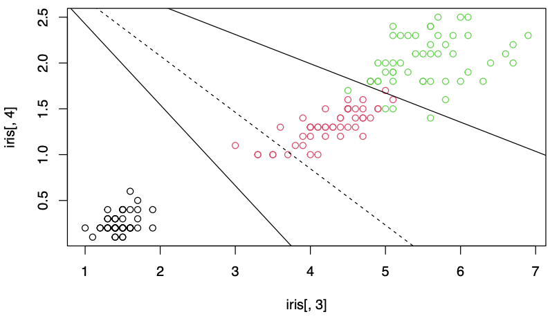
Boundaries
The boundaries of classification regions can be obtained by equating pairwise discriminants and finding the intersection points. For instance, the boundary of \(R_1\) and \(R_2\) consists of \(\boldsymbol{x}\) satisfying \(d_1(\boldsymbol{x} ) = d_2 (\boldsymbol{x} )\).
If there are \(g\) populations, there are \(\binom{g}{2}\) hyperplanes forming the boundaries. Each can be found by equating two discriminant functions \(d_i(\boldsymbol{x} ) = d_j (\boldsymbol{x} )\). The discriminant function \(d_i(\boldsymbol{x})\) can be estimated by sample discriminants \(\hat{d}_k(\boldsymbol{x})\), thus form the borders of the sample classification regions.
The dashed line in the plotted area is redundant: the classification of any point by the line would be re-evaluated by the other two partition lines. But the dashed line would not be redundant in slightly expanded areas outside the plot.
Unequal Covariance
Two-classes
When two subpopulations do not have a common covariance matrix, \(\boldsymbol{\Sigma} _1 \ne \boldsymbol{\Sigma} _2\), their population density ratio has the form
\[\begin{split}
\begin{aligned}
\ln \frac{f_{1}(\boldsymbol{x})}{f_{2}(\boldsymbol{x})}=& \frac{1}{2} \ln \frac{\left|\boldsymbol{\Sigma}_{2}\right|}{\left|\boldsymbol{\Sigma}_{1}\right|}-\frac{1}{2}\left[\boldsymbol{x}^{\top}\left(\boldsymbol{\Sigma}_{1}^{-1}-\boldsymbol{\Sigma}_{2}^{-1}\right) \boldsymbol{x}\right.\\
&\left.-\boldsymbol{x}^{\top} \boldsymbol{\Sigma}_{1}^{-1} \boldsymbol{\mu}_{1}+\boldsymbol{x}^{\top} \boldsymbol{\Sigma}_{2}^{-1} \boldsymbol{\mu}_{2}-\boldsymbol{\mu}_{1}^{\top} \boldsymbol{\Sigma}_{1}^{-1} \boldsymbol{x}+\boldsymbol{\mu}_{2}^{\top} \boldsymbol{\Sigma}_{2}^{-1}\right) \\
&\left.+\boldsymbol{\mu}_{1}^{\top} \boldsymbol{\Sigma}_{1}^{-1} \boldsymbol{\mu}_{1}-\boldsymbol{\mu}_{2}^{\top} \boldsymbol{\Sigma}_{2}^{-1} \boldsymbol{\mu}_{2}\right]
\end{aligned}
\end{split}\]
The minimum ECM classification regions becomes
\[
R_{1}:-\frac{1}{2} {\color{teal}{\boldsymbol{x}}}^{\top}\left(\boldsymbol{\Sigma}_{1}^{-1}-\boldsymbol{\Sigma}_{2}^{-1}\right) {\color{teal}{\boldsymbol{x}}}+\left(\boldsymbol{\mu}_{1}^{\top} \boldsymbol{\Sigma}_{1}^{-1}-\boldsymbol{\mu}_{2}^{\top} \boldsymbol{\Sigma}_{2}^{-1}\right) {\color{teal}{\boldsymbol{x}}}-k \geq \ln \left(\frac{c(1 \vert 2)}{c(2 \vert 1)} \cdot \frac{p_{2}}{p_{1}}\right)
\]
where \(k=\frac{1}{2}\left(\boldsymbol{\boldsymbol{\mu}}_{1}^{\top} \boldsymbol{\Sigma}_{1}^{-1} \boldsymbol{\boldsymbol{\mu}}_{1}-\boldsymbol{\boldsymbol{\mu}}_{2}^{\top} \boldsymbol{\Sigma}_{2}^{-1} \boldsymbol{\boldsymbol{\mu}}_{2}\right)+\frac{1}{2} \ln \frac{\left|\boldsymbol{\Sigma}_{1}\right|}{\left|\boldsymbol{\Sigma}_{2}\right|}\).
Now the terms involving \(\boldsymbol{x}\) are quadratic in \(\boldsymbol{x}\). Hence the function is called quadratic discriminant function. In particular, if \(\boldsymbol{\Sigma} _1 = \boldsymbol{\Sigma} _2\), then the quadratic term is zero, the remaining terms reduce to the linear classification function in the equal variance case.
The sample classification rule for \({\color{teal}{\boldsymbol{x}_{0}}}\) to \(\pi_1\) is
\[
-\frac{1}{2} {\color{teal}{\boldsymbol{x}_{0}}}^{\top}\left(\boldsymbol{S}_{1}^{-1}-\boldsymbol{S}_{2}^{-1}\right) {\color{teal}{\boldsymbol{x}_{0}}}+\left(\bar{\boldsymbol{x}}_{1}^{\top} \boldsymbol{S}_{1}^{-1}-\bar{\boldsymbol{x}}_{2}^{\top} \boldsymbol{S}_{2}^{-1}\right) {\color{teal}{\boldsymbol{x}_{0}}}-\hat{k} \geq \ln \left(\frac{c(1 \vert 2)}{c(2 \vert 1)} \cdot \frac{p_{2}}{p_{1}}\right)
\]
where \(\hat{k}=\frac{1}{2}\left(\bar{\boldsymbol{x}}_{1}^{\top} \boldsymbol{S}_{1}^{-1} \bar{\boldsymbol{x}}_{1}-\bar{\boldsymbol{x}}_{2}^{\top} \boldsymbol{S}_{2}^{-1} \bar{\boldsymbol{x}}_{2}\right)+\frac{1}{2} \ln \frac{\left|\boldsymbol{S}_{1}\right|}{\left|\boldsymbol{S}_{2}\right|}\).
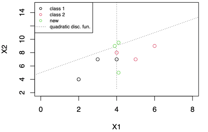
Since the function involves is quadratic in \(\boldsymbol{x}\), the regions partitions the space to three pieces in general. One region, say, \(R_2\), could be in the middle of two \(R_1\) sections, or vice versa, e.g. hyperbola in 2-d case. This sometimes does not make sense.
Multi-classes
Apply the multi-classes classification rule under equal cost that minimizes ECM
\[
R_{k}=\left\{\boldsymbol{x}: p_{k} f_{k}(\boldsymbol{x}) \geq p_{i} f_{i}(\boldsymbol{x}), \forall\ i \ne k\right\}
\]
to the normal density:
\[\begin{split}\begin{aligned}
\ln(p_i f_i (\boldsymbol{\boldsymbol{x}}))
&= \ln \left(p_{i}\right)-\frac{p}{2} \ln (2 \pi)-\frac{1}{2} \ln \left|\boldsymbol{\Sigma}_i\right|-\frac{1}{2}\left(\boldsymbol{x}-\boldsymbol{\mu}_{i}\right)^{\top} \boldsymbol{\Sigma}_i^{-1}\left(\boldsymbol{x}-\boldsymbol{\mu}_{i}\right)\\
&= d_i^Q(\boldsymbol{x}) -\frac{p}{2} \ln (2 \pi)
\end{aligned}\end{split}\]
where \(d_i^Q(\boldsymbol{x})\) is the quadratic discrimination score
\[
d_{i}^{Q}(\boldsymbol{x})=\ln \left(p_{i}\right)-\frac{1}{2} \ln \left|\boldsymbol{\Sigma}_{i}\right|-\frac{1}{2}\left(\boldsymbol{x}-\boldsymbol{\mu}_{i}\right)^{\top} \boldsymbol{\Sigma}_{i}^{-1}\left(\boldsymbol{x}-\boldsymbol{\mu}_{i}\right), \quad i=1, \cdots, g
\]
To avoid ties, we usually require \((\boldsymbol{\mu} _i, \boldsymbol{\Sigma} _i) \ne (\boldsymbol{\mu} _j, \boldsymbol{\Sigma} _j)\) for all \(i \ne j\).
The classification region becomes
\[\begin{split}\begin{aligned}
R_{k}
&=\left\{\boldsymbol{x}: d_{k}^{Q}(\boldsymbol{x}) \geq d_{i}^{Q}(\boldsymbol{x}), \text { for all } i \neq k\right\} \\
&=\left\{\boldsymbol{x}: d_{k}^{Q}(\boldsymbol{x})=\max \left\{d_{1}^{Q}(\boldsymbol{x}), \cdots, d_{g}^{Q}(\boldsymbol{x})\right\}\right\}
\end{aligned}\end{split}\]
In sample classification rule, \(d_i^Q(\boldsymbol{x})\) is estimated.