Minimum Knapsack
Problem
- Input
There are \(n\) kinds of items, each kind of item has a value \(v_i\), integer weight \(w_i\), and infinite number of it.
- Objective
Choose a subset of items that maximize value while adhering to knapsack weight constraint \(b\).
Let \(x_i\) be the number of \(i\)-th kind of items in the knapsack, the objective is
Analysis
Since the objective function and constraint are both linear in \(x_i\), this is a linear programming problem.
Subproblems
The subproblem can be defined by \(k\) and \(y\), where \(k\) is the first \(k \le n\) kinds of items, and \(y\le b\) is the weight constraint. When \(k=n,y=b\) then this is the original problem. The computational order can be \(k=1,\ldots,n\) and for each \(k\), \(y=1,\ldots,b\).
Iterative Relation
Let \(F_{k,y}\) the total optimized value of subproblem \((k,b)\). Consider the last category \(k\). We can either select none, or select one, at each selection step. The iterative relation is
The initialization is
The last line covers the situation when \(y-w_k<0\) in the iterative relation. Since it is not a feasible solution, we assign \(-\infty\) value to it.
Another way of writing the iterative relation is
But to compute \(F_{k,y}\), this way needs \(\left\lfloor\frac{y}{w_{k}}\right\rfloor\) iterations over \(x_k\), which can be \(O(b)\), unlike \(O(1)\) two-value comparison in the previous way.
Algorithm
The DP table can be computed as discussed above. Here we discuss how to trace the solution \(x_i, \ldots, x_n\).
First we define a label function \(i_{k,y}\). Let \(i_{k,y}\) be the maximum label of items added in the solution of subproblem \((k,y)\). We can find that
And the initialization is
For instance, for the problem
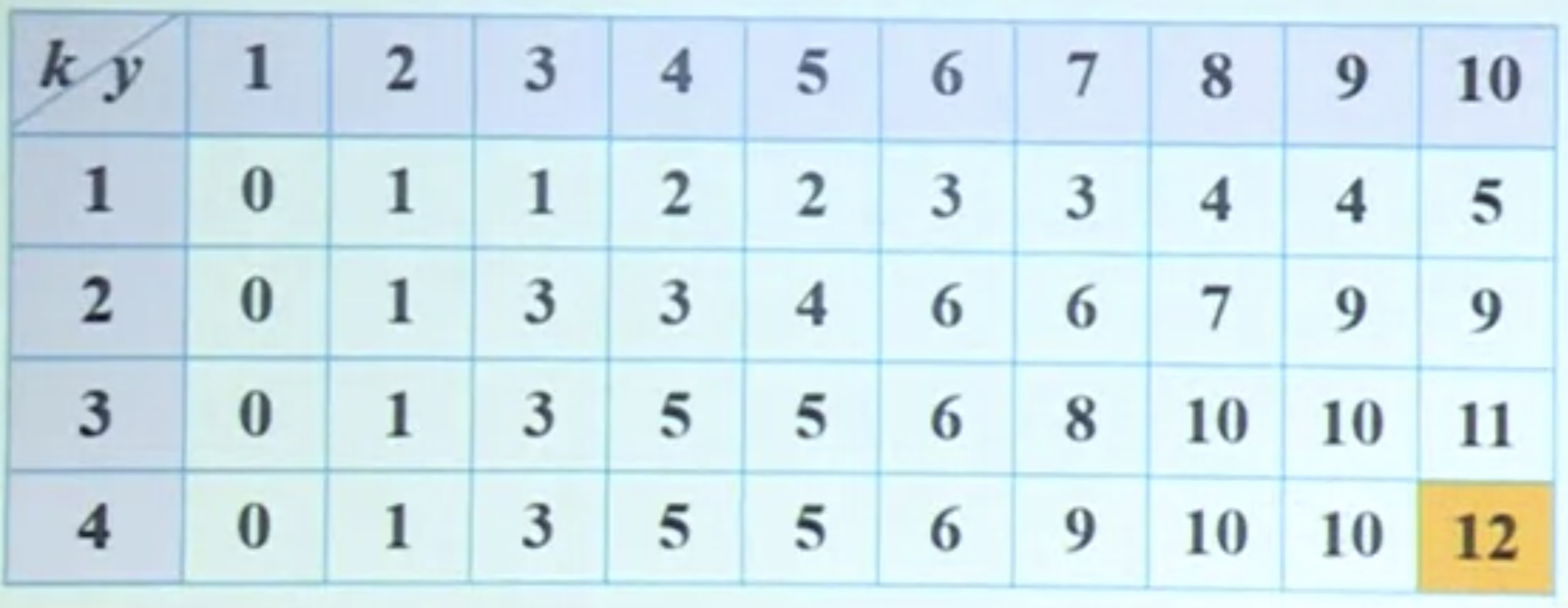
The DP table \(F_{k,y}\) is

Fig. 33 DP table
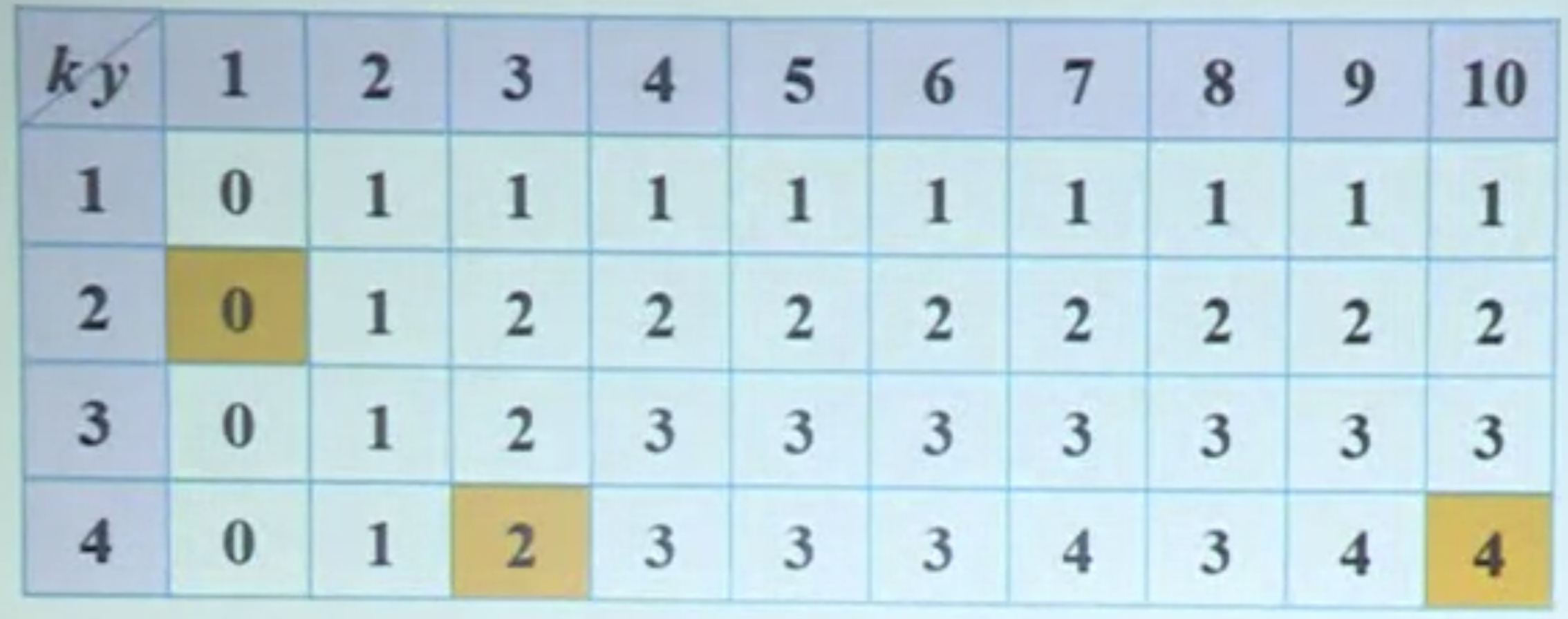
and the track table with values \(i_{k,y}\) is

Fig. 34 Track table
To track a solution, we start from the right bottom entry,
Since \(i_{4,10} = 4\), this implies \(x_4 \ge 1\). We then go to \(i_{4,10-w_4} = i_{4,3}\), i.e. subproblem \((4,3)\)
Since \(i_{4,3}=2\), this implies \(x_3, x_4=0\), and \(x_2 \ge 1\). We then go to \(i_{2,3-w_2} = i_{2,0}\)
Since \(i_{2,0}=0\), this implies \(x_2=1, x_1=0\).
Hence, the solution is \(x_1=0, x_2=1, x_3=0, x_4=1\).
The algorithm is
Knapsack: Track Solution
input: table \(i_{j,k}\)
output: soluiton \(x_1, \ldots, x_k\)
initialize \(x_j\leftarrow 0\) for \(j=1\) to \(n\)
\(y\leftarrow b, j\leftarrow n\) // start from bottom right
\(j \leftarrow i_{j,y}, x_j \leftarrow 1, y\leftarrow y-w_j\) // go to subproblem
while \(i_{j,y} = j\), // add another \(j\)
\(y \leftarrow y-w_j\)
\(x_j \leftarrow x_j + 1\)
If \(i_{j,y}\ne 0\) then goto 3
Complexity
There are \(O(nb)\) entries, and each entry takes \(O(1)\) for the two-value max comparison.
So total \(O(nb)\).
Note that this is pseudo-polynomial time, since \(b\) is not a problem size.
Extensions
Number Constraints
For each kind of item, there is a maximum number to be added.
One common example is \(n_i=1\), i.e. we can only select none or one for a kind of item.
The iterative relation becomes
Multiple Knapsacks
There are multiple knapsack, each has weight constraint \(b_j\).