Penalized Regression
Aka regularized regression, or shrinkage method.
In penalized regression, we penalize the maginitude of \(\boldsymbol{\beta}\).
where \(\lambda \in [0, \infty]\) controls the penalty term. Since we want smaller \(\left\| \boldsymbol{\beta} \right\| _p\), penalized regression is often known as shrinkage method.
Different \(p\)-norms correspond to different problems and interpretation. In many cases we want to penalize \(\boldsymbol{\beta}\), for instance, when
high multicollinearity exists
\(n < d\), then \(\boldsymbol{X} ^{\top} \boldsymbol{X}\) is not invertible
variable selection, want some \(\hat{\beta}_j=0\)
Ridge Regression
Ridge regression uses \(L_2\) norm. The objective function is
Equivalently, ridge regression can be written as solving
The optimizer is
Effect of \(\lambda\)
When \(\lambda = 0\), we obtain \(\hat{\boldsymbol{\beta} }_{\text{ridge} } = \hat{\boldsymbol{\beta} }_{\text{OLS} }\)
When \(\lambda = \infty\), we obtain \(\hat{\boldsymbol{\beta} }_{\text{ridge} } = 0\)
In general, as \(\lambda\) increases
bias \(\left\| \mathbb{E} [\hat{\boldsymbol{\beta} }_{\text{ridge} }] - \boldsymbol{\beta} \right\|\) increases
variance \(\operatorname{tr}\left( \operatorname{Cov}\left( \hat{\boldsymbol{\beta} }_{\text{ridge} } \right) \right)\) decreases
The overall mean squared error \(\mathbb{E} [\left\| \hat{\boldsymbol{\beta} }_{\text{ridge} } - \boldsymbol{\beta} \right\|_2^2 ]\) can be reduced for a range of \(\lambda\) compared to \(\hat{\boldsymbol{\beta} }_{\text{OLS} }\). In fact, this range always exists. See here.
Note that Ridge regression will include all variables by having \(\hat{\boldsymbol{\beta} _i} = 0\) for all coefiicients. Hence no effect of varibale selection.
Application:
When \(\boldsymbol{X} ^{\top} \boldsymbol{X}\) in not invertible or close to singularity.
Interpretattion of adding \(\lambda \boldsymbol{I}\) to \(\boldsymbol{X} ^{\top} \boldsymbol{X}\):
want this term large enough to make \((\boldsymbol{X} ^{\top} \boldsymbol{X} + \lambda \boldsymbol{I} ) ^{-1}\) invertible
want this term small enough to have a reasonable estimate
when there exists multicollinearity issue, Ridge regression provides more stable estimation.
Ridge regression estimation generally shrinks the estimated parameters from the ordinary least squares estimates.
For example, if we assume orthogonal design \(\boldsymbol{X} ^{\top} \boldsymbol{X} = \boldsymbol{I}\), then the ith estimator \(\hat{\beta}_{i}^{\text {ridge }}=\frac{1}{\lambda+1}\hat{\beta}_{i}^{\text{LS} }\).
LASSO Regression
In variable selection problem, it is often desirable to have a small subset of non-zero estimates of \(\beta_i\) for the purpose of model interpretation, especially when \(p\) is large. Replacing the 2-norm \(\left\| \boldsymbol{\beta} \right\|_2\) in Ridge regression model by 1-norm \(\left\| \boldsymbol{\beta} \right\|_1\) does a good job in variable selection.
LASSO (Least Absolute Shrinkage and Selection Operator) optimizes
Equivalently, LASSO regression can be written as solving
A characteristic of LASSO estimator \(\hat{\boldsymbol{\beta} }_{\text{Lasso} }\) is its sparsity. The solution would have many zero entry \(\hat{\beta}_i\) = 0. This is because the shape of \(L_1\) norm in \(d\)-dimensional space is pointy.
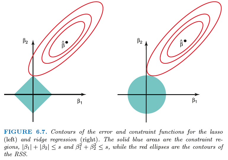
Fig. 76 Comparison of Ridge and Lasso [Introduction to Statistical Learning]
As \(\lambda\) increases (or \(s\) decreases), more and more coefficients are shrinked toward 0.
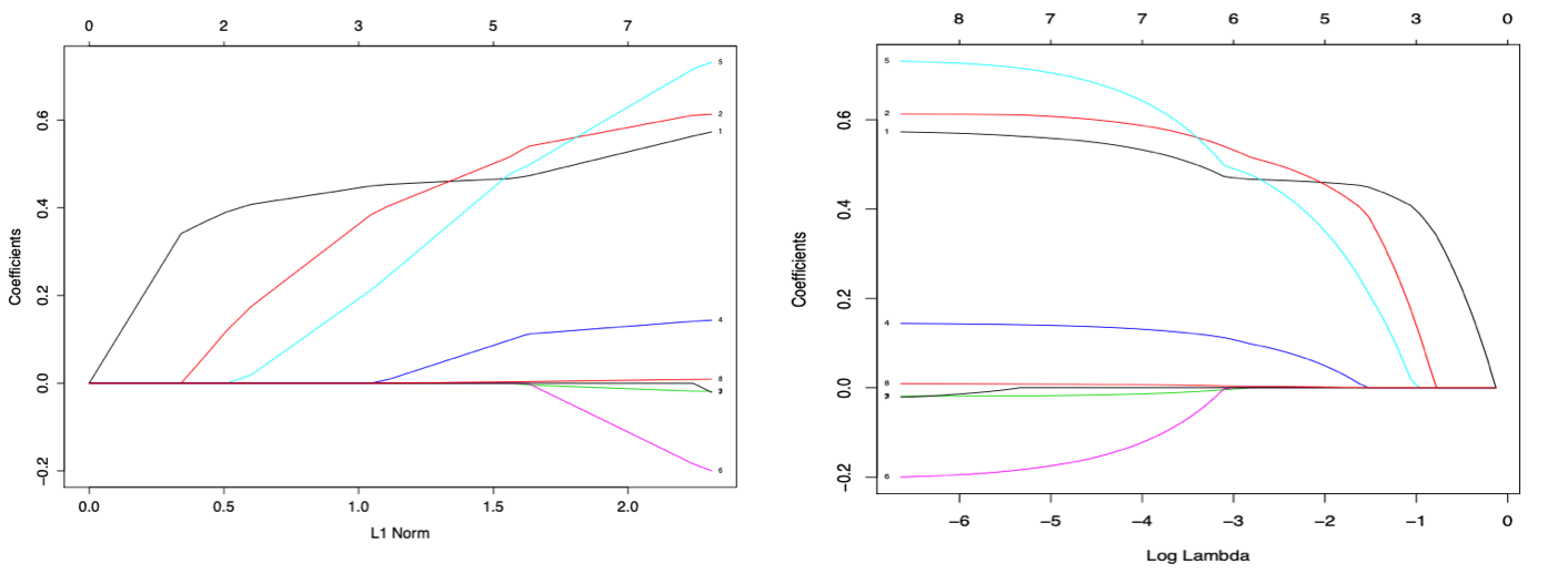
Fig. 77 How the coefficients are shrinked according to \(s\) (left) and \(\lambda\) (right). In R, use plot(glmnet(x,y))) or plot(glmnet(x,y)), xvar='lambda'). [Wang 2021]
To choose the optimal value of \(\lambda\), we can use cross-validation.
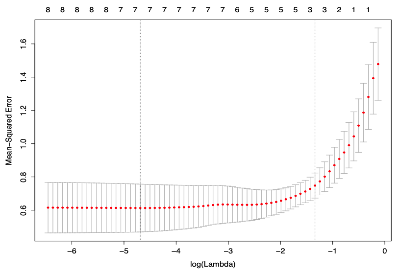
Fig. 78 Cross validation of LASSO [Wang 2021]
For the cv.glmnet(x, y) function in R
lambda.minmeans the value of lambda that gives minimum mean squared errors.lambda.1semeans the largest value of lambda such that error is within 1 standard error of the minimum MSE.
Elastic Net
As a combination of Ridge and LASSO regressions, Elastic Net optimizes
Or in another common notation,
If a few covariates \(X_i\) are correlated,
Ridge tends to keep them similar sized,
LASSO tends to keep one of them,
E-Net at certain value tends to either keep them all in, or leave them all out.
Optimization algorithms (e.g., coordinate descent) are used to obtain parameter estimates efficiently.
Comparison
We can generate data to compare the above methods.
# source: Wang 2021

library(MASS) # use lm.ridge
library(glmnet)

# simulate data
set.seed(1)
n = 50
p1 = 10 # number of signals
p2 = 20 # number of noise
X = matrix(rnorm(n*(p1+p2)), n, p1+p2)
c1 = 0.5 + (runif(10))/2 # signals coefficients 0.5 + U(0,1)/2
c2 = (runif(20))*3/10 # noise coefficients U(0,1)*3/10
Y = X[,1:10]%*%c1 + X[,11:30]%*%c2 + rnorm(n)
hist(c(c1,c2),nclass=15) # coefficients

# models
LSfit = lm(Y~X) # least squares
lm.ridge(Y~X, lambda=25) # Ridge, need to specify lambda
lassofit = cv.glmnet(X, Y) # Lasso, get a bunch of lambdas from cross validation
netfit = cv.glmnet(X, Y, alpha=0.5) # Elastic Net, need to specify alpha only. Defaulte alpha=1, i.e. Ridge

# estiamted coefficients
points(rep(2,30),lm(Y~X)$coef[2:31],cex=.5, col=c(rep(2,10),rep(1,20)), pch=c(rep(2,10),rep(1,20)))
points(rep(3,30),lm.ridge(Y~X,lambda=25)$coef,cex=.5, col=c(rep(2,10),rep(1,20)), pch=c(rep(2,10),rep(1,20)))
points(rep(4,30),coef(lassofit,s="lambda.min")[2:31],cex=.5, col=c(rep(2,10),rep(1,20)), pch=c(rep(2,10),rep(1,20)))
points(rep(5,30),coef(lassofit,s="lambda.1se")[2:31],cex=.5, col=c(rep(2,10),rep(1,20)), pch=c(rep(2,10),rep(1,20)))
points(rep(6,30),coef(netfit,s="lambda.1se")[2:31],cex=.5, col=c(rep(2,10),rep(1,20)), pch=c(rep(2,10),rep(1,20)))
title("True coefficients, LS, Ridge, Lasso.min, Lasso.1se, Net.1se")
The coefficients of signals are in \({\color{red}{\Delta}}\) and that of noise are in \(\circ\). We can see that
LS fail to separte signal and noise
Ridge has shrinkage edffect but also mix some signal with noise
Lasso with 1se and E-net do a good job
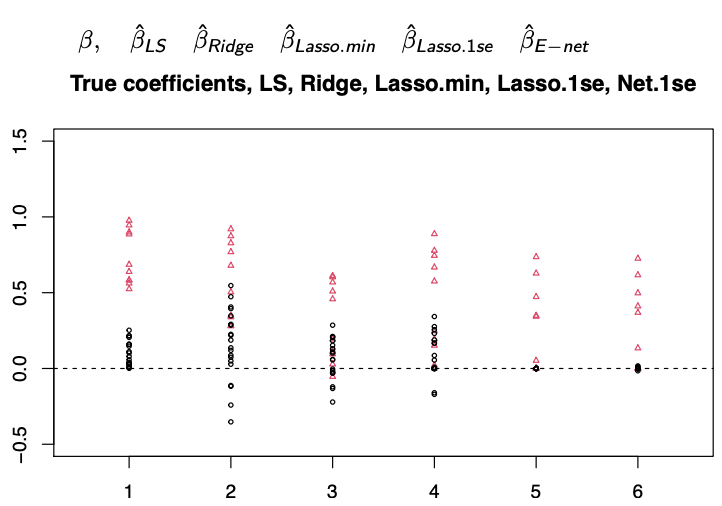
Fig. 79 Comparison of estiamted coefficients [Wang 2021]