Confusion Matrix
condition positive \(+\) |
condition negative \(-\) |
|
|---|---|---|
predicted positive \(\widehat{+}\) |
TP |
FP |
predicted negative \(\widehat{-}\) |
FN |
TN |
Metrics defined by column total (true condition)
true positive rate, recall, sensitivity, probability of detection, power.
false negative rate, miss rate
false positive rate, fall-out, probability of false alarm, type I error
true negative rate, specificity, selectivity
Metrics defined by row total (predicted condition)
false discovery rate
precision
Metrics defined by overall table
accuracy
Probability that the predicted result is correct
\[\operatorname{\mathbb{P}}\left( \widehat{+} \cap +\right) + \operatorname{\mathbb{P}}\left( \widehat{-} \cap -\right) = \frac{\mathrm{TP}+\mathrm{TN}}{\text{total population}} \]Not useful when the two classes are of very different sizes. For example, assigning every object to the larger set achieves a high proportion of correct predictions, but is not generally a useful classification.
prevalence
Proportion of true condition in a population
\[ \operatorname{\mathbb{P}}\left( + \right) = \frac{\mathrm{TP}+\mathrm{FN}}{\text{total population}} \]\(F_1\) score
The \(F_1\) score is the harmonic mean of precision and recall. Hence, it is often used to balance precision and recall.
\[F_1 = \frac{1}{\text{precision}^{-1} + \text{recall}^{-1}} = \frac{\mathrm{TP}}{\mathrm{TP} + \frac{1}{2}\left( \mathrm{FP} + \mathrm{FN} \right) }\]Closer to 1, better.
Macro \(F_1\) score
Macro \(F_1\) score extends \(F_1\) score for multiple binary labels, or multiple classes. It is computed by first computing the F1-score per class/label and then averaging them. Aka Macro F1-averaging.
\[ \text{Macro } F_1 = \frac{1}{K} \sum_{k=1}^K F_{1, k} \]where \(K\) is the number of classes/labels.
Matthews correlation coefficient
Simply the correlation coefficient between predicted binary values and actual binary values. Can also be computed as
\[ \mathrm{MCC}=\frac{\mathrm{TP} \times \mathrm{TN}-\mathrm{FP} \times \mathrm{FN}}{\sqrt{(\mathrm{TP}+\mathrm{FP})(\mathrm{TP}+\mathrm{FN})(\mathrm{TN}+\mathrm{FP})(\mathrm{TN}+\mathrm{FN})}} \in [-1, 1] \]
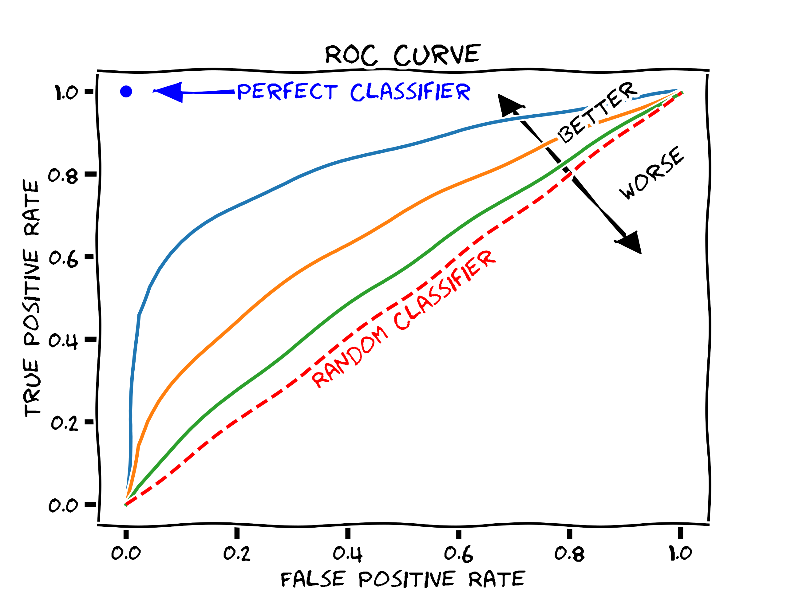
ROC curve: receiver operating characteristics curves,
y-axis: true positive rate, aka TPR, recall, sensitivity
x-axis: false positive rate, aka FPR, 1-specificity
varying a parameter controlling the discrimination between positives and negatives
classifiers with curves pushing more into the upper left-hand corner are generally considered more desirable. 45 degree line is random guessing.
AUC: area under the curve, close to 1 is good. 0.5 is random guessing. If there are \(n\) output pairs of (FPR, TPR), then area can be computed as
\[ \operatorname{AUC} = \frac{1}{2} \sum_{k=1}^n (\operatorname{FPR}_k - \operatorname{FPR} _{k-1})(\operatorname{TPR} _k + \operatorname{TPR} _{k-1}) \]