Decision Tree
Decision trees are a top-down approach for classification.
Start with all data in a single node (the root)
Find the best “question” for partitioning the data at a given node into two sub-nodes, according to some criteria
Repeat for each newly generated nodes
Stop when there is insufficient data at each node, or when the best question isn’t helpful enough
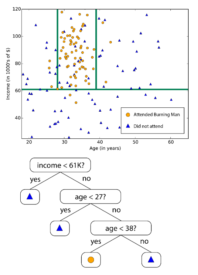
Fig. 90 A simple example of decision tree [Livescue 2021]
We need to specify
Choice of questions for the splits
Criterion for measuring the “best” question at each node
Stopping criterion
Decision tree can also be used for regression.
Regression Tree for estimating a continuous response variable: Take an average as the prediction in each partition region.
Classification Tree for classifying a categorical response variable: Take a vote as the prediction in each partition region.
Learning
Algorithm
Suppose we have a fixed, discrete set of questions. Let \(Q_{j\ell}\) denote the \(\ell\)-th pre-determined question for feature \(j\).
Starting at the root, try splitting each node into two sub-nodes,
For each feature \(X_j\), evaluate questions \(Q_{j1}, Q_{j2} \ldots\); let \(X^*, Q^*\) denote the best feature and question respectively
If \(Q^*\) isn’t sufficiently helpful in improving some partition metric, call the current node a leaf
Otherwise, split the current node into two sub-nodes according to the answer to question \(Q^*\)
Stop when all nodes are either too small to split or have been marked as leaves (there is no “good enough” question anymore). Each leaf node represents a class.
Partition Metrics
To evaluate question quality, we need some partition metrics.
Maximum Purity
Suppose
\(\Omega\) is the proposed clustering,
\(C\) is the ground-truth clustering
\(w_k\) is a proposed cluster with label \(k\)
\(c_j\) is a ground-truth cluster with ground truth label \(j\)
Then the purity of the proposed clustering \(\Omega\) and the ground-truth \(C\) is defined as
That is, for each proposed cluster \(w_k\), we find a true cluster \(c_j\) that has the maximum-cardinality intersection with \(w_k\). We can view \(w_k\) has a “predicted” label \(k\leftarrow j\). (??)
- Properties
in \((0,1)\)
biased toward finer clusterings (purity \(=1\) if each example is in its own cluster), so this measure makes sense for comparing clusterings with a given fixed number of clusters
Maximum Normalized Mutual Information
Define
\(p(k, j) = \frac{\left|\omega_{k} \cap c_{j}\right|}{N}\) as the probability that a randomly chosen example belongs to proposed cluster \(w_k\) and ground-truth cluster \(c_j\).
\(p_\Omega (k) = \frac{\left\vert w_k \right\vert}{N}\) as the probability that a randomly chosen example belongs to proposed cluster \(w_k\)
\(p_C(j)= \frac{\left\vert c_j \right\vert}{N}\) likewise
The mutual information of induced from the joint distribution \(p(k,j)\) is
and we can define entropies \(H(\Omega)\) and \(H(C)\).
Finally, the normalized mutual information is
Properties
Ranges from 0 and 1
Mutual information alone would also favor over-clustering
Entropies in the denominator act as penalty for over-clustering
Note
For unlabelled data, we can use maximum likelihood and minimum entropy.
Maximum Likelihood
The best question at a node is the maximum likelihood one, i.e. the one that maximizes the likelihood of the two newly formed (left and right) groups of data points
Often, the models for the left and right nodes are each a single Gaussian
Note that the best question should always improve likelihood somewhat.
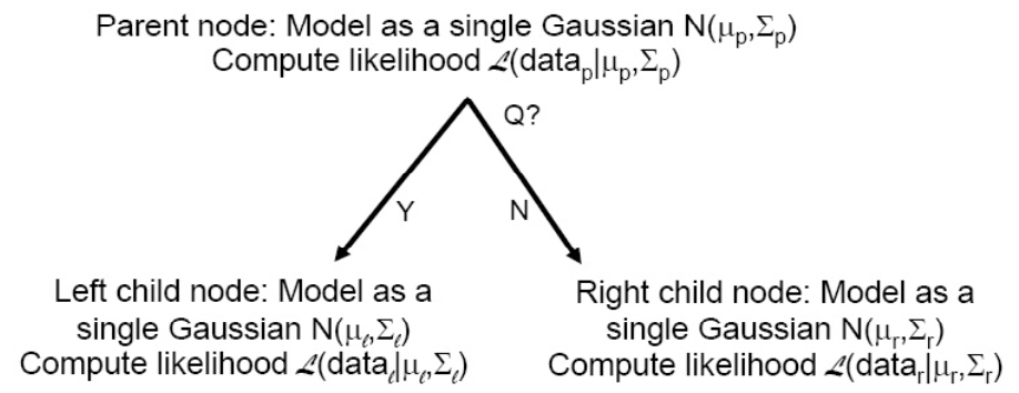
Fig. 91 Evaluating question quality by maximum likelihood
Minimum Entropy
Another common criterion is to minimize node entropy (uncertainty measured in bits).
Recall that if \(X\) is a discrete random variable taking one of \(n\) values with probabilities \(p_{1}, \ldots, p_{n}\) , respectively, then the entropy of
Minimum RSS
For regression, i.e. \(y\) is a continuous variable, we can use residual sum of square (RSS) as a splitting criteria. For two sub nodes \(R_m\) where \(m = 1, 2\) by some splitting rule, the RSS is
Stoping Criteria
When should we stop partitioning? Or how to determine the size/depth of the tree?
Simple Heuristics Based
Leaves too small: data at a node has fewer than some threshold samples
Best question does not improve likelihood significantly (e.g. 10%)
Out of time/memory for more nodes
Cross-validation
Measure likelihood with different tree sizes on a held-out (development) data set, choose the tree size that maximizes likelihood
Measure downstream performance on held-out data set, on some task of interest
Pruning
If there are too many nodes (size of the tree), the tree model may overfit. To avoid it, we can prune the tree, i.e. remove some splits.
Cost complexity pruning
Aka weakest link pruning. Take regression tree as an example.
We first define the cost of a tree \(T\)
The optimal pruned tree is selected by cross validation (like selecting \(\lambda\) in LASSO).
Split the data into \(K\) folds.
Construct a range of \(\alpha\) values. For each \(\alpha\),
Fit a tree on \((K-1)\) folds by minimizing \(\operatorname{cost}_\alpha(T)\).
Evaluate the fitted tree on the hold-out fold, compute RSS.
Repeat for \(K\) folds, compute average RSS.
select best \(\alpha^*\) that minimizes average RSS. Build a tree using full data by minimizing \(\operatorname{cost} _{\alpha^*}(T)\). This is the output tree.
Comment
Larger tree, easier to overfit
If underlying relation is linear, then linear models probably works better. If non-linear, tree-based methods may work better.
Random Forest
Group of weaker classifiers can form a stronger one!
Learning
Given a data set of \(n\) observations and \(p\) features.
Boostrap sampling rows and columns to build \(T\) trees
Select a size \(n\) random sample with replacement from the original sample data to grow a classification tree (same size with original data set, but some observations appear multiple times)
At each node of the tree, randomly select \(m<p\) input variables to split the node.
If \(m=p\), then called ‘bagging’
Usually \(m \sim \sqrt{p}\). may perform better than bagging.
Decision: For the \(k\)-th observation, the classification rule is by the most votes of trees or by taking the average (as in regression) where the \(k\)-th observation is not used in the tree construction (out-of-bag, OOB).
Each observation is OOB for about one third of the trees (thus no validation sample is needed)
The average of the error rate of the \(n\) observations is the OOB error rate of the forest.
Error rate of the forest increases with the correlation between trees. Then the more uncorrelated the trees, the better. Inter-tree correlation increases with \(m\).
Variable Importance
OOB observations also used to evaluate variable importance. Each variable is randomly permuted to check its impact on some cost measures, e.g. MSE, Gini Node Purity.
The mean decrease in the cost across all trees is reported.
Note that if a variable has very little predictive power, shuffling may lead to a slight decrease in cost due to random noise. This in turn can give rise to small negative importance scores, which can be essentially regarded as equivalent to zero importance.