Spectral Clustering¶

Spectral clustering methods use a similarity graph (as in graph-based dimensionality reduction) to represents the data points, then apply spectral (eigenvector-based) methods on certain graph matrices associated with the connectivity of $G$, to divide the graph into connected sub-graphs.

Similar to graph-based representation learning, there are three steps for spectral clustering. Given a data set.

Define a similarity measure
Construct a similarity graph, and obtain
- Adjacency matrix
- Laplacian matrix
- …
Run graph cut algorithm on graph matrices with some objectives.

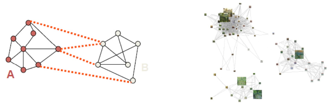
Fig. 123 Divide the graph into sub-graphs [D. Sontag]¶

Similarity Graphs¶

Formally, we have data points $\boldsymbol{x}_{1}, \ldots, \boldsymbol{x}_{n}$, Consider some similarity measures $s_{i j}$ or dissimilarity measures $d_{ij}$. We create a graph $G=(V,E)$, add one node $v_i$ for each data point $\boldsymbol{x}_i$, and unweighted or weighted edges by some criterions.

$\varepsilon$-neighborhood graph: add edge $(v_i, v_j)$ if $d_{ij} \le \varepsilon$
- Advantages: Geometrically motivated, the relationship is naturally symmetric.
- Disadvantages: Often leads to graphs with several connected components, difficult to choose $\epsilon$.
$k$-NN: add edge $(v_i,v_j)$ if $v_j$ is a $k$-NN of $v_i$ or vice versa, according to $d_{ij}$
- Advantages: Easier to choose; does not tend to lead to disconnected graphs.
- Disadvantages: Less geometrically intuitive.
Mutual $k$-NN: add edge $(v_i,v_j)$ if $v_i$ is a $k$-NN of $v_j$ and vice versa. It works well for sub-graphs with different densities.
Fully connected: add edge $(v_i,v_j)$ with weight $w_{ij} = s_{ij}$ or some function of $s_{ij}$.

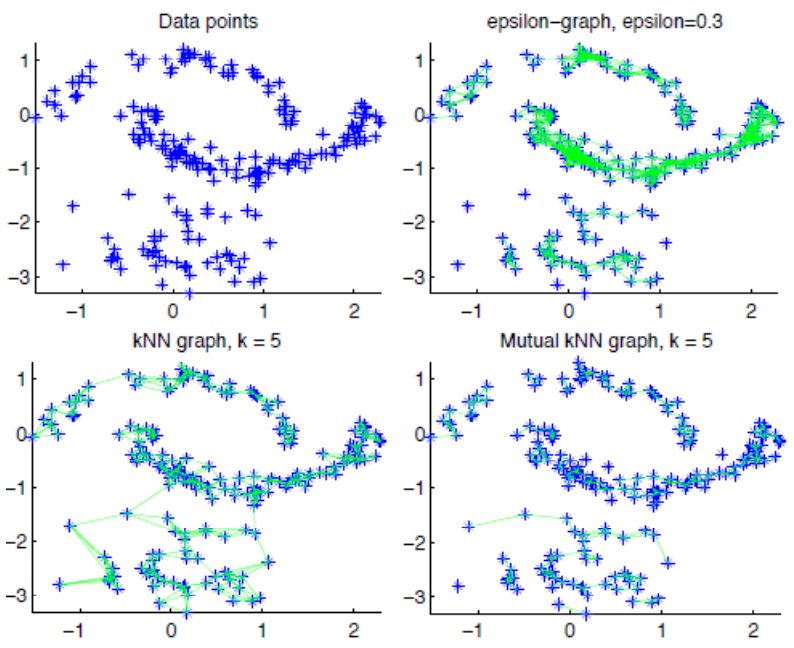
Fig. 124 Comparison of three types of graphs [von Luxburg]¶

We mainly consider bisection ($K=2$) and unweighted case.

Adjacency Matrix-based¶

Recall that an adjacency matrix contains binary entries of connection relation between any two nodes. Sometimes we can extend it to be the matrix of edge weights (similarities).

Degree (considering weights) $\operatorname{deg} (i)=\sum_{j} a_{i j} = \operatorname{RowSum}_i (A)$
Volume of a set $S$ of nodes $\operatorname{vol}(S)=\sum_{i \in S} \operatorname{deg} (i)$.

Property¶

Let the eigen-pairs of an binary adjacency matrix $\boldsymbol{A}$ be $(\lambda_i, \boldsymbol{v}_i)$, where $\lambda_1 \le \ldots \le \lambda_{N_v}$ (not necessarily distinct).

Fact (Spectrum of graph adjacency matrices)

In the case of a graph $G$ consisting of two $d$-regular graphs joined to each other by just a handful of vertices,

the two largest eigenvalues $\lambda_1, \lambda_2$ will be roughly equal to $d$, and the remaining eigenvalues will be of only $\mathcal{O} (d^{1/2})$ in magnitude. Hence, there is a gap in the spectrum of eigenvalues, namely ‘spectral gap’.
the second eigenvector $\boldsymbol{v} _2$ are expected to have large positive entires on vertices of one $d$-‘regular’ graphs, and large negative entires on the vertices of the other. For details, see stochastic block models.

Bisection¶

Using this fact, to find two clusters in the data set, we can compute eigenvalues and eigenvectors of $\boldsymbol{A}$, then find the largest positive and largest negative entries in the 2nd eigenvector. Their respective neighbors are declared to be two clusters.

For instance, in the plots below, We see that

The first two eigenvalues are fairly distinct from the rest, indicating the possible presence of two sub-graphs.
The first eigenvector appears to suggest a separation of the 1st and 34th actors, and some of their nearest neighbors, from the rest of the actors.
The second eigenvector in turn provides evidence that these two actors, and certain of their neighbors, should themselves be separated.

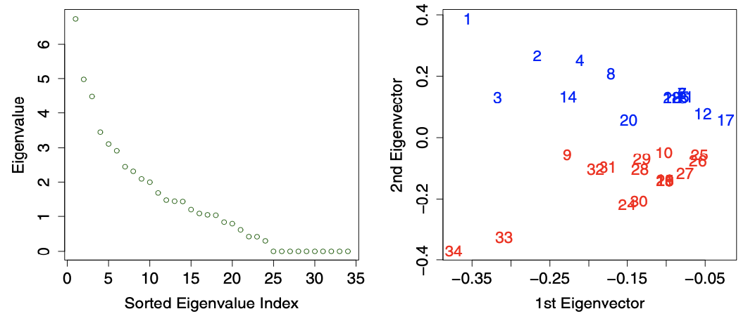
Fig. 125 Spectral analysis of the karate club network. Left: $\left\vert \lambda_i \right\vert$. Right: $\boldsymbol{v} _1, \boldsymbol{v} _2$, colored by subgroups. [Kolaczyk 2009]¶

For unkonwn $k$, we can

Look for a spectral gap to determine $k$
Run $k$-means clustering using the first $k$ eigenvectors to determine assignment

Pros and Cons¶

Cons

In reality, graphs are far from regular, so this method does not work well
The partitions found through spectral analysis will tend to be ordered and separated by vertex degree, since the eigenvalues will mirror quite closely the underlying degree distribution. Normalizing the adjacency matrix to have unit row sums is a commonly proposed solution.

For an analysis of this method, i.e. how well the discretization of empirical $\boldsymbol{v} _2$ gives the correct binary label, see the section.

Laplacian Matrix-based¶

Recall that the graph Laplacian matrix is defined as $\boldsymbol{L} = \boldsymbol{D} -\boldsymbol{A}$ where $\boldsymbol{D}$ is diagonal matrix of degrees.

Let the eigen-pairs of $\boldsymbol{L}$ be $(\lambda_i, \boldsymbol{v}_i)$, where $\lambda_1 \le \ldots \le \lambda_{N_v}$ (not necessarily distinct).

Property¶

Fact (Spectrum of graph Laplacian matrices): A graph $G$ will consist of $K$ connected components if and only $\lambda_1 = \ldots = \lambda_K = 0$ and $\lambda_{K+1} > 0$.

Therefore, if we suspect a graph $G$ to consist of nearly $K=2$ components, then we expect $\lambda_2$ to be close to zero.

Definitions

The ratio of the cut defined by $(S, \bar{S})$ is the ratio between the number of across-part edges and the number of vertices in the smaller component.

\[\phi(S, \bar{S}) = \frac{\left\vert E(S, \bar{S}) \right\vert}{ \left\vert S \right\vert}\]
The isoperimetric number of a graph $G$ is defined as the smallest ratio of all cuts.

\[\phi(G)=\min _{S \subset V:|S| \leq N_{v} / 2} \phi(S, \bar{S})\]

The ratio is a natural quantity to minimize in seeking a good bisection of $G$. Unfortunately, this minimization problem to find $S$ for $\phi(G)$, aka ratio cut, is NP-hard. But the isoperimetric number is closely related to $\lambda_2$

Cheeger’s Inequality: The isoperimetric number $\phi(G)$ is bounded by $\lambda_2$ as

\[ \frac{\lambda_{2}}{2} \leq \phi(G) \leq \sqrt{\lambda_{2}}\left(2 \operatorname{deg} _{\max }-\lambda_{2}\right) \]

Thus, $\phi(G)$ will be small when $\lambda_2$ is small and vice versa.

Bisection¶

Fiedler [SAND 144] associate $\lambda_2$ with the connectivity of a graph. We partition vertices according to the sign of their entires in $\boldsymbol{v} _2$:

\[ S_F=\left\{u \in V: \boldsymbol{v} _{2}[u] \geq 0\right\} \quad \text { and } \quad \bar{S}_F=\left\{u \in V: \boldsymbol{v} _{2}[u]<0\right\} \]

The eigenvector $\boldsymbol{v} _2$ is hence often called the Fiedler vector
The eigenvalue $\lambda_2$ is often called the Fiedler value, which is also the algebraic connectivity of the graph

This method is often called spectral bisection. It can be shown that

\[ \phi(G) \leq \phi(S_F, \bar{S}_F) \leq \frac{\phi^{2}(G)}{\operatorname{deg} _{\max }} \leq \lambda_{2} \]

Fiedler bisection can be viewed as a computationally efficient approximation to finding a best cut achieving $\phi(G)$. In the example below, we see that is gives a good result, classifying all but the 3rd actor correctly.

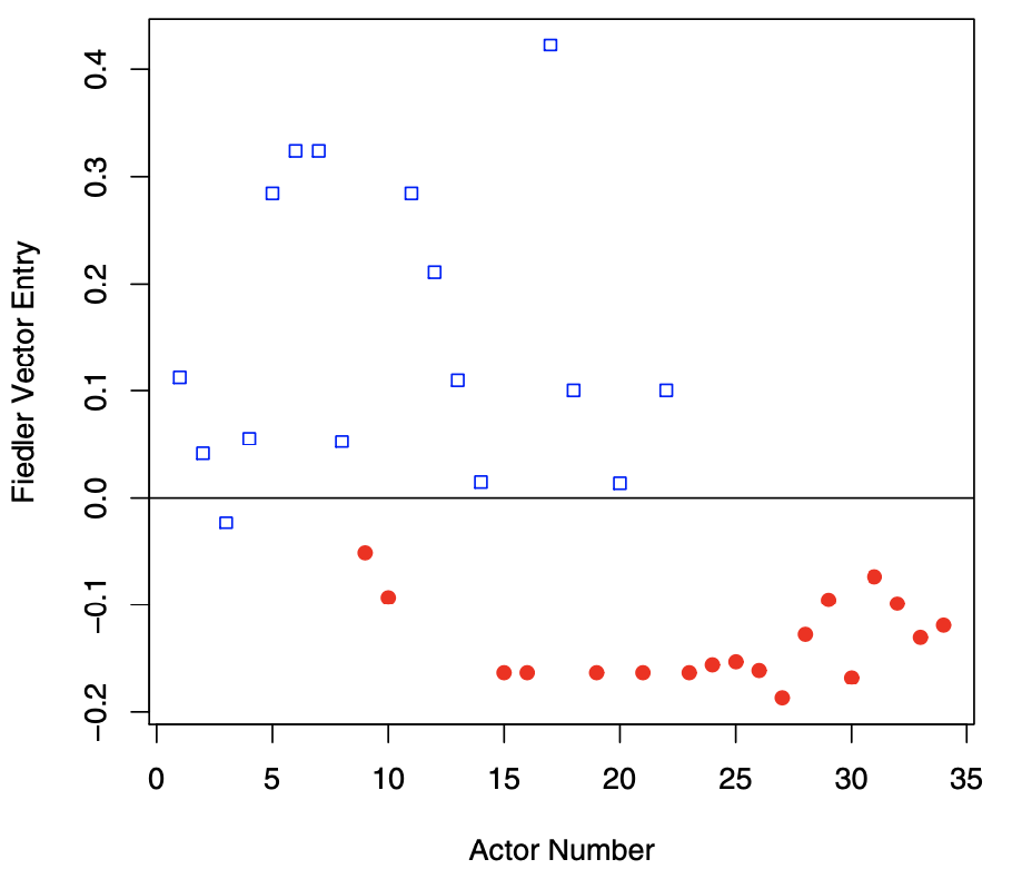
Fig. 126 Fiedler vector $\boldsymbol{v} _2$ of the karate club graph. Color and shape indicate subgroups. [Kolaczyk 2009]¶

For $K \ge 3$, apply bisection recursively.

Pros and Cons¶

Pros

Work well on bounded-degree planar graphs and certain mesh graphs [SAND 366]

Computation¶

For both of the two spectral partitioning methods above, the computational overhead is in principle determined by the cost of computing the spectral decomposition of an $N_v \times N_v$ matrix $\boldsymbol{A}$ or $\boldsymbol{L}$, which takes $\mathcal{O} (N_v^2)$ time. However, realistically,

only a small subset of extreme eigenvalues and eigenvectors are needed.
the matrices $\boldsymbol{A}$ and $\boldsymbol{L}$ will typically be quite sparse in practice.

Lanczos algorithm can efficiently solve such settings. If the graph between $\lambda_2$ and $\lambda_3$ is sufficiently large (nearly $K=2$), the spectral bisection takes $\mathcal{O} (\frac{1}{\lambda_3 - \lambda_2} N_e)$, i.e. almost linear.

Weighted Case¶

Now we consider the weighted case from optimization point of view, where weights $w_{ij} = s_{ij}$.

We define the (unnormalized) graph Laplacian as

\[\boldsymbol{L} = \boldsymbol{D} - \boldsymbol{W}\]

where

$\boldsymbol{W}$ is the similarity matrix of $s_{ij}$
$\boldsymbol{D}$ is the diagonal matrix of $\boldsymbol{W} \boldsymbol{1}$

The volume of a set $S$ of vertices extends to $\operatorname{vol}(S)= \sum_{i \in S} d_i = \sum_{i \in S} \left( \sum_{j \in N(i)} w_{ij} \right)$.

Objectives¶

Definition (Value of a cut): A cut is a partition of the graph into two sub-graphs $S$ and $\bar{S}$. The value of a cut is defined as the sum of total edge weights between the two subgraphs

\[W(S, \bar{S})=\sum_{i \in A, j \in B} w_{i j}\]

To partition the graph into $K$ subgraphs, we would like to minimize the sum of cut values between each subgraph $A_i$ and the rest of the graph:

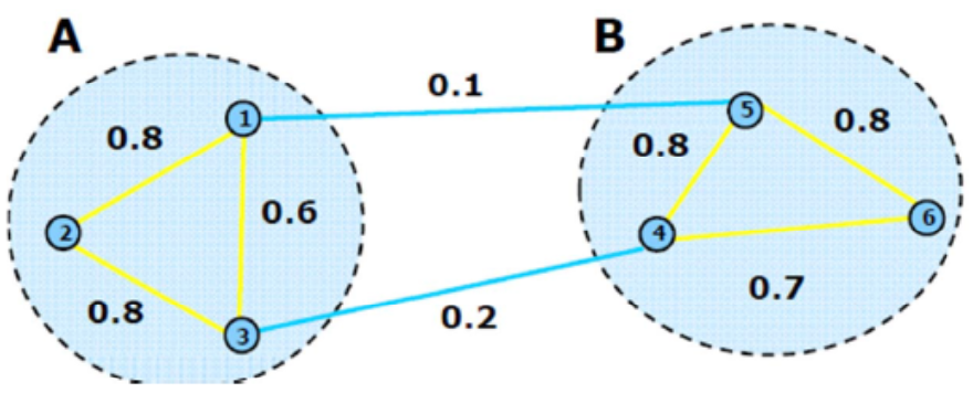
\[ \underset{S_{1}, \ldots, S_{K}}{\operatorname{min}} \frac{1}{2} \sum_{k=1}^{K} W\left(S_{k}, \bar{S}_{k}\right) \]

Fig. 127 A graph cut with $W(S,\bar{S})=0.3$ [Hamad & Biela]¶

The algorithm with the above objective function is called Min Cut, which favors isolated nodes.

Other methods with modified/normalized objectives include:

Ratio cuts $(\operatorname{RatioCut} )$ normalizes by cardinality: $\frac{1}{2} \sum_{k=1}^{K} \frac{W\left(S_{k}, \bar{S}_{k}\right)}{\left|S_{k}\right|}$
Normalized cuts $(\operatorname{Ncut})$ normalizes by volume: $\frac{1}{2} \sum_{i=1}^{k} \frac{W\left(S_{i}, \bar{S}_{i}\right)}{\operatorname{vol}\left(S_{i}\right)}$.

Bisection Min Cut¶

Recall that the bisection Min-cut objective is

\[\min_S\ W\left(S, \bar{S}\right)\]

We define a indicator vector $\boldsymbol{c} \in\{-1,1\}^{n}$, where $c_i = 1$ means data point $i$ is in cluster/subgraph $S$; otherwise cluster $\bar{S}$. Note that

\[ W\left(S, \bar{S}\right) = \sum_{i \in S, j \in \bar{S}} w_{i j} = \frac{1}{4}\sum_{ij} w_{ij}(c_i - c_j)^2 = \frac{1}{4} \boldsymbol{c} ^{\top} \boldsymbol{L} \boldsymbol{c} \]

The objective can be formulated as

\[\begin{split}\begin{aligned} \min_{\boldsymbol{c}} &&& \boldsymbol{c} ^{\top} \boldsymbol{L} \boldsymbol{c}\\ \mathrm{s.t.} &&& \boldsymbol{c} \in\{-1,1\}^{n} \\ \end{aligned}\end{split}\]

A relaxation of this problem is to solve for a continuous $\boldsymbol{c}$ vector instead $\boldsymbol{c} \in \mathbb{R} ^{n}$

\[\begin{split}\begin{aligned} \min_{\boldsymbol{c}} && \boldsymbol{c} ^{\top} \boldsymbol{L} \boldsymbol{c} &\\ \mathrm{s.t.} && \boldsymbol{c} &\in \mathbb{R} ^n\\ && \boldsymbol{c} ^{\top} \boldsymbol{c} &= n \\ \end{aligned}\end{split}\]

If we don’t add the $\boldsymbol{c} ^{\top} \boldsymbol{c} = n$ constraint then a trivial solution is $\boldsymbol{c} = \boldsymbol{0}$. The solution is given by the eigenvector of the eigenproblem

\[ \boldsymbol{L} \boldsymbol{c}=\lambda \boldsymbol{c} \]

The first eigenvector of $\boldsymbol{L}$ is all ones (all data in a single cluster, which is meaningless). We take the 2nd eigenvector $\boldsymbol{v} _2$ as the real-valued solution. There are several ways to decide the binary assignment

take 0 or the median value as the splitting point or,
search for the splitting point such that the resulting partition has the best objective value

Actually, this problem can be solved exactly. See the max flow section.

Bisection Normalized Cut¶

[Shi & Malik 1999]

Recall that the objective of the bisection normalized cut is

\[\min_S\ \left( \frac{W\left(S, \bar{S}\right)}{\operatorname{vol}\left(S\right)} + \frac{W\left(\bar{S}, S\right)}{\operatorname{vol}\left(\bar{S}\right)} \right)\]

Let the $\boldsymbol{c} \in\{-1,1\}^{n}$ be the assignment vector. Define $\boldsymbol{y} = (\boldsymbol{1} + \boldsymbol{x} ) - b (\boldsymbol{1} - \boldsymbol{x} )$ where $b = \frac{\operatorname{vol}(S) }{\operatorname{vol}(\bar{S})}$ such that $y_i = 2$ if $x_i=1$, and $y_i = -2b$ and $x_i = -1$. It can be shown that finding $\boldsymbol{c}$ is equivalent to solve the following optimization problem for $\boldsymbol{y}$

\[\begin{split}\begin{aligned} \min _{\boldsymbol{y} } && \frac{\boldsymbol{y} ^{\top} \boldsymbol{L} \boldsymbol{y} }{\boldsymbol{y} ^{\top} \boldsymbol{D} \boldsymbol{y} } & &&\\ \mathrm{s.t.} && \boldsymbol{y} &\in \left\{ 1, -b \right\} ^n &&\\ && \boldsymbol{y} ^{\top} \boldsymbol{D} \boldsymbol{1} &= \boldsymbol{0} && \\ \end{aligned}\end{split}\]

where the constraint $\boldsymbol{y} ^{\top} \boldsymbol{D} \boldsymbol{1} = \boldsymbol{0}$ comes from the condition of the assignment vector $\boldsymbol{x}$. However, solving for discrete combinatorial values is hard. The optimization problem is relaxed to solve for a continuous $\boldsymbol{y} \in \mathbb{R} ^n$ vector instead. The solution $\boldsymbol{y} ^*$ is given by the 2nd smallest eigenvector of the generalized eigenproblem (see the paper eq. 6-9)

\[ \boldsymbol{L} \boldsymbol{y}=\lambda \boldsymbol{D} \boldsymbol{y} \]

That is, $\boldsymbol{y} ^*$ is the 2nd smallest eigenvector of random-walk Laplacian $\boldsymbol{L} ^{\mathrm{rw}} = \boldsymbol{D} ^{-1} \boldsymbol{L}$. Moreover, if we set $\boldsymbol{z} ^* = \boldsymbol{D} ^{1/2} \boldsymbol{y}^*$, then $\boldsymbol{z} ^*$ is the second smallest eigenvector of symmetric normalized Laplacian $\boldsymbol{L} ^\mathrm{sym}= \boldsymbol{D} ^{-1/2} \boldsymbol{L} \boldsymbol{D} ^{-1/2}$. See properties of graph Laplacians.

We then find a splitting point to decide assignment with the methods introduced in Min-cut.

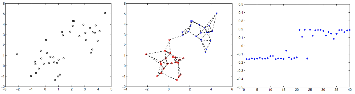
Fig. 128 $\operatorname{Ncut}$ for a data set of $40$ points.¶

More Clusters¶

Option 1: Recursively apply the 2-cluster algorithm
Option 2: For $K$ clusters, treat the smallest $K-1$ eigenvectors (excluding the last one) as a reduced-dimensionality representation of the data, and cluster these eigenvectors. The task will be easier if the values in the eigenvectors are close to discrete, like the above case.

Applications¶

Comparison to $k$-means¶

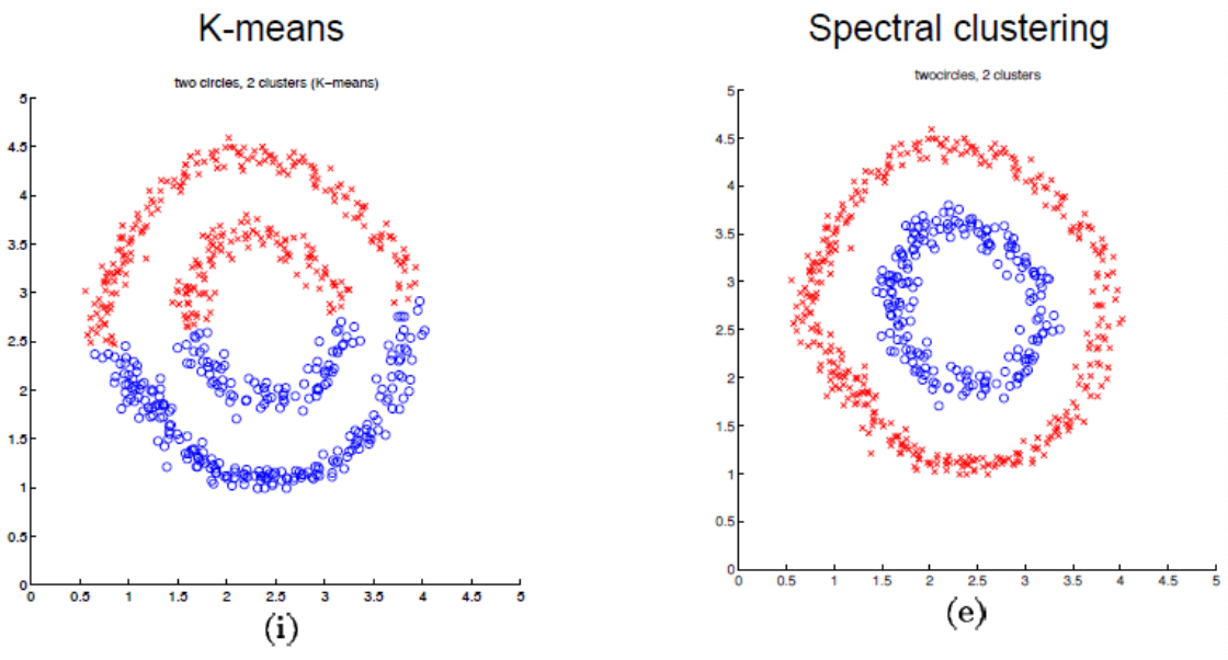
Fig. 129 $k$-means vs spectral clustering on double rings data set [Ng, Jordan, & Weiss]¶

Image Segmentation¶

For an image, we can view each pixel $i$ as a graph vertex, and the similarity depends on pixel content (color intensity) $f_i$ and pixel location $x_i$:

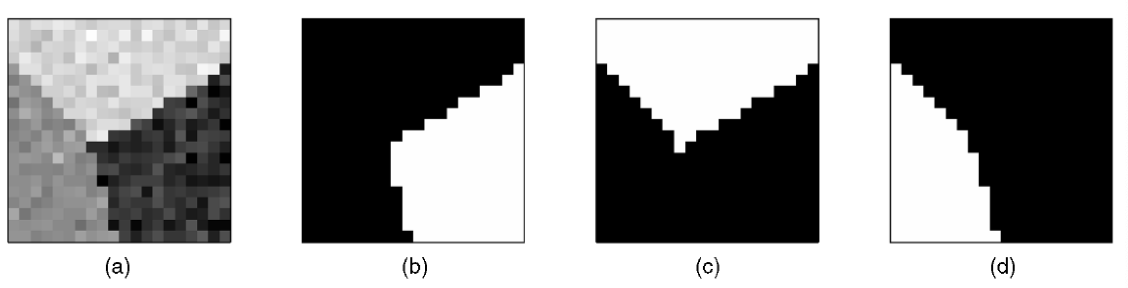
\[\begin{split} w_{i j}= \left\{\begin{array}{ll} \exp \left\{ -\left(\frac{1}{2 \pi \sigma^{2}}\|f_i-f_j\|^{2}+\frac{1}{2 \pi \tau^{2}}\|x_i- x_j\|^{2}\right) \right\}, & \text { if } \left\vert x_i-x_j \right\vert< \varepsilon \\ 0, & \text { otherwise } \end{array}\right. \end{split}\]

Fig. 130 Spectral clustering for image segmentation [Shi & Malik]¶

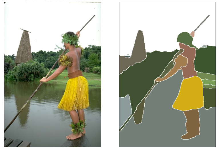
Fig. 131 Spectral clustering for image segmentation [Arbel ́aez et al.]¶

Speech Separation¶

Speech separation (into speakers): Similar to image segmentation, where a “pixel” is a cell of a spectrogram. Darkness corresponds to amount of frequency at that time.

Fig. 132 Spectral clustering for speech separation [Bach & Jordan]¶

Stochastic Block Models¶

Aka planted partition model.

Adjacency Matrix¶

Consider a perfect case: a graph consisting of $k$ clusters of equal size $\frac{n}{k}$, each cluster is complete and there are no across-cluster edges, then the spectral decomposition of $\boldsymbol{A}$ is

\[\begin{split} \boldsymbol{A} = \left[\begin{array}{ccc} \boldsymbol{1} \boldsymbol{1} ^{\top} & 0 & 0\\ 0 & \ddots & 0 \\ 0 & 0 & \boldsymbol{1} \boldsymbol{1} ^{\top} \end{array}\right], \quad \boldsymbol{U} = \frac{1}{\sqrt{n/k}} \left[\begin{array}{ccc} \boldsymbol{1} & 0 & 0\\ 0 & \ddots & 0 \\ 0 & 0 & \boldsymbol{1} \end{array}\right] \boldsymbol{Q}, \quad \boldsymbol{\Lambda} = \frac{n}{k} \boldsymbol{I} \end{split}\]

where $\boldsymbol{1}$ are a vector of size $\frac{n}{k}$. $\boldsymbol{Q}$ is an orthogonal transform (does not change distance between a pair of embeddings).

In practice, $\boldsymbol{A}$ is not that perfect. How imperfect $\boldsymbol{A}$ can be?

Consider a stochastic block model (SBM), $k=2$ clusters (each cluster has size $\frac{n}{2}$), and

\[\begin{split} \mathbb{P} (A_{ij} = 1) = \left\{\begin{array}{ll} p, & \text { if $i, j$ in same cluster} \\ q, & \text { if $i, j$ in different cluster} \\ \end{array}\right. \end{split}\]

Usually $p >q$. Then the expectation of the random adjacency matrix is

\[\begin{split} \mathbb{E} [\boldsymbol{A}] = \left[\begin{array}{cc} p \boldsymbol{1} \boldsymbol{1} ^{\top} & q \boldsymbol{1} \boldsymbol{1} ^{\top} \\ q \boldsymbol{1} \boldsymbol{1} ^{\top} & p \boldsymbol{1} \boldsymbol{1} ^{\top} \\ \end{array}\right] = \frac{p+q}{2} \boldsymbol{1}_n \boldsymbol{1}_n ^{\top} + \frac{p-q}{2} \left[\begin{array}{cc} \boldsymbol{1} \\ -\boldsymbol{1} \end{array}\right] [\boldsymbol{1} ^{\top} \ -\boldsymbol{1} ^{\top}] \end{split}\]

and $\mathbb{E} [\boldsymbol{A}]$ has rank 2 and two non-zero eigenvalues

\[\begin{split}\begin{aligned} \lambda_1 &= \frac{p+q}{2}n & \boldsymbol{v} _1 &= \frac{1}{\sqrt{n}} \boldsymbol{1} _n \\ \lambda_2 &= \frac{p-q}{2}n & \boldsymbol{v} _2 &= \frac{1}{\sqrt{n}}\left[\begin{array}{cc} \boldsymbol{1} \\ -\boldsymbol{1} \end{array}\right] \\ \end{aligned}\end{split}\]

Hence, to give labels for 2-clustering, we can discretize $\boldsymbol{v} _2$ of $\mathbb{E} [\boldsymbol{A}]$ according to the signs of its entries. However, we only observe $\boldsymbol{A}$ rather than $\mathbb{E} [\boldsymbol{A}]$. Is the second eigenvector $\boldsymbol{\hat{v}} _2$ of $\boldsymbol{A}$ a good estimator for $\boldsymbol{v} _2$ of $\mathbb{E} [\boldsymbol{A}]$?

Analysis¶

Suppose we know the parameters $p, q$. Now we analyze the discretization performance by quantify some ‘distance’ between $\boldsymbol{v} _2$ and $\boldsymbol{\hat{v}}_2$.

First, we can write $\boldsymbol{A} = \mathbb{E} [\boldsymbol{A} ] + (\boldsymbol{A} - \mathbb{E} [\boldsymbol{A} ] )$ where the second term is noise. If noise $=0$, then the second eigenvectors of observed $\boldsymbol{A}$ is that of $\mathbb{E} [\boldsymbol{A}]$, which is $\frac{1}{\sqrt{n}} \left[\begin{array}{cc} \boldsymbol{1} \\ -\boldsymbol{1} \end{array}\right]$, whose its discretization perfectly reveals the label.

But the second eigenvector is hard to analyze (since its computation depends on the 1st eigenvector, which is also random). We introduce an equivalent analysis: compute the first eigenvector of $\boldsymbol{A} - \frac{p+q}{2} \boldsymbol{1}_n \boldsymbol{1}_n ^{\top}$, denoted $\boldsymbol{\hat{u}}$. And assign the label according to the sign of the entries in $\boldsymbol{\hat{u}}$. Some interpretation

avoid computing the first eigenvector which is not informative
approximately equivalent to compute the top eigenvector of the ‘centered’ version of $\boldsymbol{A}$: $\boldsymbol{C} \boldsymbol{A} \boldsymbol{C}$ where $\boldsymbol{C} = \boldsymbol{I} - \frac{1}{n}\boldsymbol{1} \boldsymbol{1} ^{\top}$.

We expect $\boldsymbol{\hat{u}} \approx \frac{1}{\sqrt{n}} \left[\begin{array}{cc} \boldsymbol{1} \\ -\boldsymbol{1} \end{array}\right]$. To analyze the error, let

truth: $\boldsymbol{M} = \mathbb{E} [\boldsymbol{A}] - \frac{p+q}{2} \boldsymbol{1}_n \boldsymbol{1}_n ^{\top} = \frac{p-q}{2} \left[\begin{array}{cc} \boldsymbol{1} \\ -\boldsymbol{1} \end{array}\right] [\boldsymbol{1} ^{\top} \ -\boldsymbol{1} ^{\top}]$
observed: $\widehat{\boldsymbol{M}} = \boldsymbol{A} - \frac{p+q}{2} \boldsymbol{1}_n \boldsymbol{1}_n ^{\top}$.
perturbation: $\boldsymbol{H} = \widehat{\boldsymbol{M}} - \boldsymbol{M} = \boldsymbol{A} - \mathbb{E} [\boldsymbol{A} ]$.

By applying Davis-Kahan theorem to SBM and use the distance measure defined there, let $r=1$, then

\[ \operatorname{dist}(\hat{\boldsymbol{u}}, \boldsymbol{u} ) = \left\| \hat{\boldsymbol{u}} \hat{\boldsymbol{u}}^{\top} - \boldsymbol{u} \boldsymbol{u} ^{\top}\right\|_2 \le \frac{\left\| \boldsymbol{A} - \mathbb{E} [\boldsymbol{A} ] \right\| }{\frac{p-q}{2} n - 0 - \left\| \boldsymbol{A} - \mathbb{E} [\boldsymbol{A}] \right\| } \]

Hence if $p \gg q$, then the error is low. Can we quantify $\left\| \boldsymbol{A} - \mathbb{E} [\boldsymbol{A} ] \right\|$? By Bernstein inequality, for $p > q \ge \frac{b \log n}{n}$,

\[ \frac{\left\| \boldsymbol{A} - \mathbb{E} [\boldsymbol{A} ] \right\| }{\frac{p-q}{2} n - \left\| \boldsymbol{A} - \mathbb{E} [\boldsymbol{A}] \right\|} \le \mathcal{O} \left( \frac{\sqrt{np \log n}}{(p-q)n} \right) \]

Therefore, when $(p-q)n \gg \sqrt{n p \log n}$, discretizing $\boldsymbol{\hat{u}}$ approximately recover $\boldsymbol{u}$.

On distance measure

If $\operatorname{dist}(\boldsymbol{u} , \hat{\boldsymbol{u} }) =\left\| \hat{\boldsymbol{u}} \hat{\boldsymbol{u}}^{\top} - \boldsymbol{u} \boldsymbol{u} ^{\top}\right\|_2$ is small, then $\left\vert \langle \boldsymbol{u} , \hat{\boldsymbol{u}} \rangle \right\vert$ is large, but some entires of $\hat{\boldsymbol{u}}$ might have opposite sign as $\boldsymbol{u}$. Hence, it is better to use other distance measure, e.g. $\left\| \cdot \right\| _\infty$, as developed by Abbe, Fan, Wang [2020].

On lower bound of $p, q$

The lower bound $\frac{b\log n}{n}$ is to ensure the graph is connected, since most algorithms applied only to relatively dense graphs [link pg.3]. Also see here and here.

When $p = \frac{a \log n}{n} , q = \frac{b \log n}{n}$, (i.e., sparse regime), then $d_i = \mathcal{O} (\log n)$ (‘constant’ degree). Need $a-b \gg \sqrt{a}$ for the algorithm to successfully detect cluster.
When $p = \frac{a}{n}, q=\frac{b}{n}$ and $a - b \ge 2 \sqrt{a + b}$, then it is possible to detect cluster that is correlated with true cluster, otherwise impossible. [Mossel, Newman, Sly 2015]

Data Science Handbook

Spectral Clustering¶

Similarity Graphs¶

Adjacency Matrix-based¶

Property¶

Bisection¶

Pros and Cons¶

Laplacian Matrix-based¶

Property¶

Bisection¶

Pros and Cons¶

Computation¶

Weighted Case¶

Objectives¶

Bisection Min Cut¶

Bisection Normalized Cut¶

More Clusters¶

Applications¶

Comparison to \(k\)-means¶

Image Segmentation¶

Speech Separation¶

Stochastic Block Models¶

Adjacency Matrix¶

Analysis¶