Graph-based Spectral Methods
PCA, CCA, MDS are linear dimensionality reduction methods. The lower-dimensional linear projection preserves distances between all points.
If our data lies on a nonlinear manifold (a topological space locally resembling Euclidean space), then we need non-linear dimensionality reduction methods. Many of them are extended from MDS, that extends to a variety of distance/similarity measures. They only preserve local distance/neighborhood information along nonlinear manifold.
In general, there are three steps:
Define some similarity/distance measure between data points \(d(\boldsymbol{x}_i ,\boldsymbol{x}_j)\).
Induce a graph from the \(n \times d\) data set \(\boldsymbol{X}\)
nodes are the data points
add edge \(e(i,j)\) if the distance \(d(\boldsymbol{x}_i,\boldsymbol{x}_j)\) satisfy certain criteria, e.g. \(d<\varepsilon\), \(k\)-NN, or mutual \(k\)-NN.
Perform spectral methods on some graph matrices, such as adjacency matrix, weights matrix, Laplacian matrix, etc, to obtain the embedding \(\boldsymbol{Z} _{n \times d}\) that preserve some property in the original space.
Examples: Isomap, maximum variance unfolding, locally linear embedding, Laplacian eigenmaps.
The obtained embeddings can then be used as input for clustering, e.g. \(k\)-means. Essentially, we look for clustering on the manifold, rather than the original space, which makes more sense.
Isomap
[Tenenbaum et al. 2000]
For a manifold in a high-dimensional space, it may NOT be reasonable to use Euclidean distance to measure the pairwise dissimilarity of points. Geodesic distance along the manifold may be more appropriate.
Isomap is a direct extension of MDS where Euclidean distances are replaced with estimated geodesic distances along the manifold, i.e. it tries to “unfold” a manifold and preserve the pairwise geodesic distances.
Learning
Isomap algorithm:
Construct a graph where node \(i\) corresponds to input example \(\boldsymbol{x}_i\), and nodes \(i\) and \(j\) are connected by an edge if \(\boldsymbol{x}_i, \boldsymbol{x}_j\) are nearest neighbors (by some definition) with edge weight being the Euclidean distance \(d_{ij} = \left\| \boldsymbol{x}_i -\boldsymbol{x}_j \right\|\).
For each \(i,j\) in the graph, compute pairwise distance \(\Delta_{i j}\) along the shortest path in the graph (e.g., using Dijkstra’s shortest path algorithm) as the estimated geodesic distance.
Perform MDS for some dimensionality \(k\), taking the estimated geodesic distances \(\Delta_{i j}\) as input in place of Euclidean distances.
The output is the \(k\)-dimensional projections of all of the data points \(\boldsymbol{z}_i\) such that the Euclidean distances in the projected space approximate the geodesic distances on the manifold.
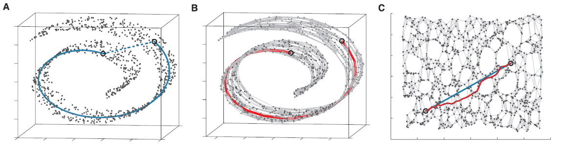
Fig. 103 Isomap with \(d=3,k=2\). The blue line is the real geodesic distance and the red line is estimated. [Livescu 2021]
Pros Cons
Pros
As the data set size increases, isomap is guaranteed to converge to the correct manifold that the data was drawn from, under certain conditions (e.g. no holes)
Cons
Can be sensitive to the neighborhood size used in graph construction, or equivalently to the noise in the data.
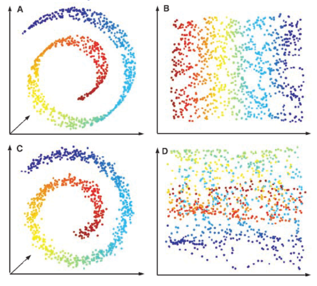
Fig. 104 Isomap fails when there are noises [Livescu 2021]
Can’t handle holes in the manifold. Geodesic distance computation can break. This is because the two points (even with the same color/label) sit in opposite to the hole have large geodesic distance on the manifold, which leads to large Euclidean distance in the projected space.
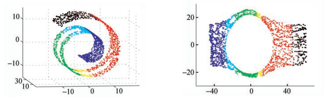
Fig. 105 Isomap fails when there are holes [Livescu 2021]
Laplacian Eigenmaps
Unlike isomap where the edge weights are local Euclidean distances, Laplacian eigenmaps define edge weights in another way.
Learning
Construct an graph \(G = (V, E)\) from data \(\boldsymbol{X}\). Add edge \((i, j)\) if \(\boldsymbol{x}_i\) and \(\boldsymbol{x}_j\) are close, in the sense that
\(\left\| \boldsymbol{x}_i - \boldsymbol{x}_j \right\| < \epsilon\), or
\(n\)-nearest-neighbors
Define edge weights as
\[\begin{split} w_{i j}=\left\{\begin{array}{ll} \exp \left(-\left\|\boldsymbol{x}_{i}-\boldsymbol{x}_{j}\right\|^{2} / t\right), & (i, j) \in E \\ 0 & \text { otherwise } \end{array}\right. \end{split}\]where \(t\) is a hyperparameter like temperature. As \(t = \infty\), \(w_{ij} = a_{ij}\).
Define a diagonal matrix \(\boldsymbol{D}\) with \(d_{ii} = \sum_j w_{ij}\). This can be seen as the density around the node \(i\). The graph Laplacian is \(\boldsymbol{L} = \boldsymbol{D} - \boldsymbol{W}\). The \(k\)-dimensional representation \(\boldsymbol{Z}\) is given by the \(k\) bottom eigenvectors (excluding the smallest one, which is \(\boldsymbol{1}\)) for the generalized eigenvector problem
\[ \boldsymbol{L} \boldsymbol{v} = \lambda \boldsymbol{D} \boldsymbol{v} \]If \(G\) is not connected, run this step for each connected component in \(G\).
Derivation
We want to preserve locality: if two data points \(\boldsymbol{x}_i , \boldsymbol{x}_j\) are close, then their embeddings \(\boldsymbol{z}_i , \boldsymbol{z}_j\) are also close. To ensure this, the loss function is formulated as
where \(w_{ij}\) measures the closeness of \(i\) and \(j\) in \(\boldsymbol{X}\). If \(i\) and \(j\) are close in \(\boldsymbol{X}\), then \(w_{ij}\) is large, which force \(\left\| \boldsymbol{z}_i - \boldsymbol{z}_j \right\|\) to be small, i.e. \(i\) and \(j\) are close in \(\boldsymbol{Z}\). For \(i\) and \(j\) that are far away in \(\boldsymbol{X}\), don’t care. Recall that the objective is to maintain locality.
It can be shown that
Hence, our objective is now
where the first constraint prevents trivial solution \(\boldsymbol{Z} = \boldsymbol{0}\). Actually \(\boldsymbol{Z} ^{\top} \boldsymbol{D} \boldsymbol{1} = \boldsymbol{0}\) is not necessary.
The solution (\(k\) columns of \(\boldsymbol{Z}\)) is given by the bottom \(k\) eigenvectors (excluding \(\boldsymbol{1}\)) of the generalized eigenvalue problem
Or equivalently, the eigenvectors of random-walk graph Laplacian: \(\boldsymbol{L} ^{\mathrm{rw}} = \boldsymbol{D} ^{-1} \boldsymbol{L}\). See graph Laplacians for details about \(\boldsymbol{L} ^\mathrm{rw}\) and \(\boldsymbol{L} ^\mathrm{sym}\).
To see why the two constraints come from, we can first see a \(k=1\) example, i.e. projection onto a line. Suppose the projections are \(z_1, \ldots, z_n\), the problem is
Note that there are two issues
arbitrary scaling: if \(\boldsymbol{z}^*\) is an optimal solution, then a new solution \(c\boldsymbol{z}^*\) where \(0<c<1\) gives a smaller function value, contradiction. Or we say \(\boldsymbol{z} = \boldsymbol{0}\) is a trivial solution.
translational invariance: if \(\boldsymbol{z} ^*\) is an optimal solution, then a new solution \(\boldsymbol{z} ^* + c\boldsymbol{1}\) gives the same function value.
To solve these two issues, we add two constraints \(\boldsymbol{z} ^{\top} \boldsymbol{D} \boldsymbol{z} = 1\) and \(\boldsymbol{z} ^{\top} \boldsymbol{D} \boldsymbol{1} = 0\) respectively. The second constraint also removes a trivial solution \(\boldsymbol{z} = c\boldsymbol{1}\), to be introduced soon. The problem becomes
In fact, the matrix \(\boldsymbol{D}\) here is introduced by the authors in the original paper to reflect vertex importance. Actually replacing \(\boldsymbol{D}\) by \(\boldsymbol{I}\) also solve these two issues.
The solution is given by the 2nd smallest eigenvector of the generalized eigenproblem
Note that \(\boldsymbol{v} = c\boldsymbol{1}\) is an eigenvector of \(\boldsymbol{L}\) but the constraint \(\boldsymbol{z} ^{\top} \boldsymbol{D} \boldsymbol{1} =0\) removes that.
To generalize to \(k\ge 2\), we generalize the constraints to \(\boldsymbol{Z} ^{\top} \boldsymbol{D} \boldsymbol{Z} = \boldsymbol{I}\) and \(\boldsymbol{Z} ^{\top} \boldsymbol{D} \boldsymbol{1} = \boldsymbol{0}\) shown above. Note that if we move the second constraint (as in the paper), then the embedding in one of the \(k\) dimensions will be \(c \boldsymbol{1}\), hence we actually obtain \((k-1)\)-dimensional embedding, but it is also helpful to distinguish points.
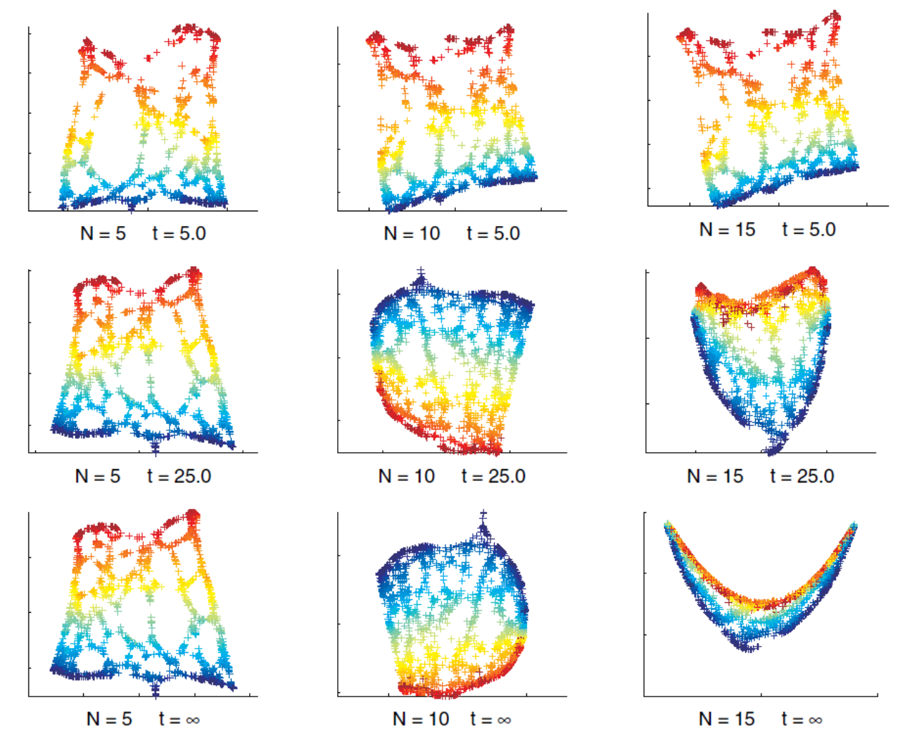
Fig. 106 Laplacian eigenmap with varing \(N\)-nearest-neighbors and temperature \(t\) [Livescu 2021]
Relation to Spectral Clustering
For the normalized cut problem in spectral clustering, the cluster label is given by the 2nd smallest eigenvector of the generalized eigen problem
which is exactly the 1-dimensional representation of Laplacian eigenmaps. In this sense, the local approach to dimensionality reduction imposes a natural clustering of data.
Seriation Problem
Suppose there are \(n\) archeological pieces \(i = 1, \ldots, n\). We want to time order them by finding some latent ordering \(\pi(i)\), given some similarity measure \(w_{ij}\). The problem can be formulated as
Solving permutation is hard. Spectral relaxation drop the permutation constraint and solve
Hope that the relative order in \(\boldsymbol{f} ^*\) can tell information about \(\pi^*\).
An example of applying MDS to seriation problem is shown below. The data is the “distances” between 9 archaeological sites from different periods, based upon the frequencies of different types of potsherds found at the sites. The MDS algorithm successfully separate years (1137, 1131) from the rest (918~1062). Moreover, we can see that in the group (918~1062), there is roughly a upward line, that aligns these seven sites chronologically. All th ese observations suggest that MDS successfully preserves the distance between among the 9 sites.
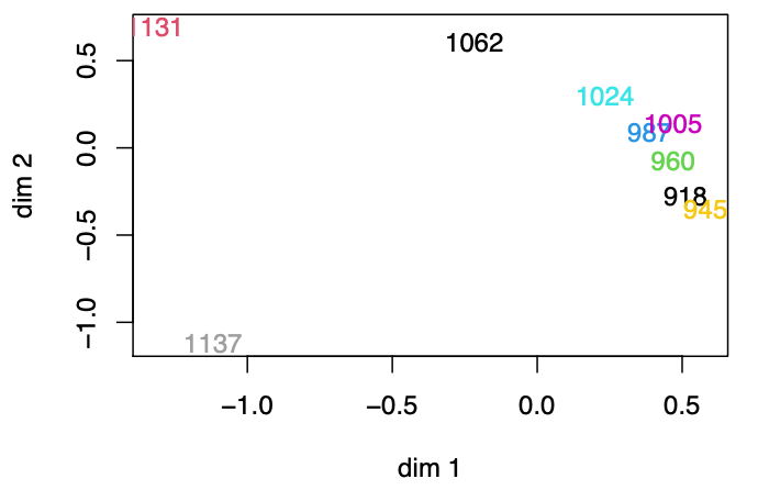
Fig. 107 Applying MDS to similarity matrix of sites.
What if we have some information, say some \(i\) is known to be in some year? Can we use this information?
Locally Linear Embedding
Locally linear embedding learns a mapping in which each point can be expressed as a linear function of its nearest neighbors.
Maximum Variance Unfolding
Maximum variance unfolding tries to maximize the variance of the data (like PCA) while respecting neighborhood relationships.
ref: https://www.youtube.com/watch?v=DW3lSYltfzo
.
.
.
.
.
.
.
.