PCA Variants
We introduce three variants of PCA: probabilistic PCA, kernel PCA, and sparse PCA.
Probabilistic PCA
Independently proposed by [Tipping & Bishop 1997, 1999] and [Roweis 1998]
Probabilistic PCA adds a probabilistic component (interpretation) to the PCA model. It provides
a way of approximating a Gaussian using fewer parameters (e.g. common noise variance).
a way of sampling from the data distribution as a probabilistic model (thus aka sensible PCA).
Objective
In a PPCA model, we first draw low dimensional \(\boldsymbol{z} \in \mathbb{R}^{k}\),
and draw \(\boldsymbol{x} \in \mathbb{R}^{d}, k \leq d\) by
where \(\boldsymbol{W} \in \mathbb{R} ^{d \times k}\)
Or equivalently,
If \(\sigma = 0\) then we get standard PCA.
By the property of multivariate Gaussian, we have
The goal is to estimate the parameter \(\boldsymbol{W} , \boldsymbol{\mu} , \sigma\) that maximize the log likelihood \(\sum_{i=1}^{n} \log p\left(\boldsymbol{x}_{i} \mid \boldsymbol{W} , \boldsymbol{\mu} , \sigma\right)\).
Learning (MLE)
Let \(\boldsymbol{C} = \boldsymbol{W} \boldsymbol{W} ^\top + \sigma^2 \boldsymbol{I}_d\). The log likelihood function is
Setting the derivative w.r.t. \(\boldsymbol{\mu}\) to \(\boldsymbol{0} \) we have
i.e. the sample mean. The solution for \(\boldsymbol{W}\) and \(\sigma^2\) is more complicated, but closed form.
where
\(\boldsymbol{U} _{d \times k}\) is the first \(k\) eigenvectors of the sample covariance matrix \(\boldsymbol{S}\)
\(\boldsymbol{\Lambda}_k\) is the diagonal matrix of eigenvalues
\(\boldsymbol{R}_k\) is an arbitrary orthogonal matrix
Properties
For \(\boldsymbol{R}_k = \boldsymbol{I}_k\) , the solution for \(\boldsymbol{W}\) is just a scaled version (by the diagonal matrix \(\boldsymbol{\Lambda} _k - \sigma^2 \boldsymbol{I} _k\)) of that of standard PCA \(\boldsymbol{U}_{d\times k}\).
\(\sigma^2_{ML}\) is the average variance of the discarded dimensions in \(\mathcal{X}\). We view the remaining dimensions as accounting for noise. Their average variance defines the common variance of the noise. The covariance is viewed as
\[\begin{split} \boldsymbol{\Sigma}=\boldsymbol{U}\left[\begin{array}{cccccccc} \lambda_{1} & \ldots & 0 & \ldots & \ldots & \ldots \\ & \ddots & 0 & \ldots & \ldots & \ldots \\ 0 & \ldots & \lambda_{k} & \ldots & \ldots & \ldots \\ 0 & \ldots & 0 & \sigma^{2} & 0 & \ldots \\ & & & & \ddots & \\ 0 & \ldots & \ldots & \ldots & 0 & \sigma^{2} \end{array}\right] \boldsymbol{U} ^\top \end{split}\]If \(k = d\), i.e., no dimension reduction, then the MLE for the covariance matrix \(\boldsymbol{C}\) of \(\boldsymbol{x}\) is equal to \(\boldsymbol{S}\), which is just the standard ML solution for a Gaussian distribution.
Representation
The conditional distribution of \(\boldsymbol{z}\) given \(\boldsymbol{x}\) is
where \(\boldsymbol{M} = \boldsymbol{W} ^\top \boldsymbol{W} + \sigma^2 \boldsymbol{I}_k\).
A reduced-dimensionality representation of \(\boldsymbol{x}\) is given by the estimated conditional mean
where \(\boldsymbol{M} _{ML} = \boldsymbol{W} _{ML} ^\top \boldsymbol{W} _{ML} + \sigma^2 _{ML} \boldsymbol{I}_k\).
As \(\sigma^2 _{ML} \rightarrow 0\), the posterior mean approaches the standard PCA projection \(\boldsymbol{ z } = \boldsymbol{U} ^\top (\boldsymbol{x} - \bar{\boldsymbol{x} })\)
As \(\sigma^2 _{ML}> 0\), the posterior mean “shrinks” the solution in magnitude from standard PCA. Since we are less certain about the representation when the noise is large.
Kernel PCA
Kernel PCA is a nonlinear extension of PCA where dot products are replaced with generalized dot products in feature space computed by a kernel function.
Kernelization
Linear PCA only consider linear subspaces
To improve this, we can apply feature transformation \(\boldsymbol{\phi}: \mathbb{R} ^d \rightarrow \mathbb{R} ^p\) to include non-linear features, such as \(\boldsymbol{\phi} ([x_1, x_2])= [x_1, x_1^2, x_1 x_2]\).
Then the data matrix changes from \(\boldsymbol{X}_{n \times d}\) to \(\boldsymbol{\Phi}_{n \times p}\). Then we run standard PCA on the new data covariance matrix \(\frac{1}{n} \boldsymbol{\Phi} ^\top \boldsymbol{\Phi}\).
Note that handcrafting feature transformation \(\boldsymbol{\phi}\) is equivalent to choosing a kernel function \(k(\boldsymbol{x}_1, \boldsymbol{x} _2) = \boldsymbol{\phi}(\boldsymbol{x} _1) ^\top \boldsymbol{\phi}(\boldsymbol{x} _2)\). And there are many advantages choosing kernels instead of handcrafting \(\boldsymbol{\phi}\). After choosing \(k(\cdot, \cdot)\), We can compute the new \(n \times n\) inner product matrix by \(\boldsymbol{K} = \boldsymbol{\Phi} \boldsymbol{\Phi} ^\top\), aka kernel matrix. And the \(k\)-dimensional embeddings for a data vector \(\boldsymbol{x}\) is given by
where \(\boldsymbol{A}_{n \times k}\) contains the first \(k\) eigenvectors of the kernel matrix \(\boldsymbol{K}\). That is, the projected data matrix is \(\boldsymbol{Z}_{n \times k} = \boldsymbol{K} \boldsymbol{A}\).
Derivation
Let \(\boldsymbol{C} = \frac{1}{n} \boldsymbol{\Phi} ^\top \boldsymbol{\Phi}\) be the new covariance matrix. To run standard PCA, we solve the eigenproblem
Now we show that \(\boldsymbol{w} \in \mathbb{R} ^d\) can be written as a linear combination of the transformed data vectors \(\boldsymbol{\phi} (\boldsymbol{x} _1), \ldots, \boldsymbol{\phi} _1(\boldsymbol{x}_n)\), i.e.,
To show this, substituting \(\boldsymbol{C} = \boldsymbol{\Phi} ^\top \boldsymbol{\Phi} = \frac{1}{n} \sum_{i=1}^n \boldsymbol{\phi} (\boldsymbol{x}_i ) \boldsymbol{\phi} (\boldsymbol{x}_i )^\top\) to the above equality, we have
Then, to find the \(j\)-th eigenvector \(\boldsymbol{w}_j\), it remains to find \(\boldsymbol{\alpha}_j\). Substituting the linear combination back to the eigenproblem gives
Therefore, \(\boldsymbol{\alpha} _j\) is the eigenvector of the kernel matrix \(\boldsymbol{K}\).
To find the embeddings, recall that \(\boldsymbol{w} = \boldsymbol{\Phi} ^\top \boldsymbol{\alpha}\), hence to embed a data vector \(\boldsymbol{x}\),
In fact, we don’t need the exact form of \(\boldsymbol{\phi}\) at all.
Mean normalization of \(\boldsymbol{K}\)
We’ve implicitly assumed zero-mean in the new feature space \(\mathbb{R} ^p\), but it is usually not. Hence, we should modify \(\boldsymbol{K}\) by
where \(\boldsymbol{C} = \left(\boldsymbol{I}-\frac{1}{n} \boldsymbol{1} \boldsymbol{1}^{\top}\right)\) is the centering matrix. Then we solve for the eigenvectors of \(\boldsymbol{K} ^c\)
Learning
From the analysis above, the steps to train a kernel PCA are
Choose a kernel function \(k(\cdot, \cdot)\).
Compute the centered kernel matrix \(\boldsymbol{K} ^c = (\boldsymbol{I} - \boldsymbol{u} \boldsymbol{u} ^\top )\boldsymbol{K}(\boldsymbol{I} - \boldsymbol{u} \boldsymbol{u} ^\top)\)
Find the first \(k\) eigenvectors of \(\boldsymbol{K} ^c\), stored as \(\boldsymbol{A}\).
Then
to project a new data vector \(\boldsymbol{x}\),
\[\begin{split}\begin{aligned} \boldsymbol{z} &= \boldsymbol{A} ^\top \left[\begin{array}{c} k(\boldsymbol{x} _1, \boldsymbol{x}) \\ k(\boldsymbol{x} _2, \boldsymbol{x}) \\ \vdots \\ k(\boldsymbol{x} _n, \boldsymbol{x}) \\ \end{array}\right]\\ \end{aligned}\end{split}\]to project the training data,
\[\boldsymbol{Z} ^\top = \boldsymbol{A} ^\top \boldsymbol{K} \text{ or } \boldsymbol{Z} = \boldsymbol{K} \boldsymbol{A} \]to project a new data matrix \(\boldsymbol{Y} _{m \times d}\),
\[\begin{split} \boldsymbol{Z} _y ^\top = \boldsymbol{A} ^\top \left[\begin{array}{ccc} k(\boldsymbol{x} _1, \boldsymbol{y_1}) & \ldots &k(\boldsymbol{x} _1, \boldsymbol{y_m}) \\ k(\boldsymbol{x} _2, \boldsymbol{y_1}) & \ldots &k(\boldsymbol{x} _2, \boldsymbol{y_m}) \\ \vdots &&\vdots \\ k(\boldsymbol{x} _n, \boldsymbol{y_1}) & \ldots &k(\boldsymbol{x} _n, \boldsymbol{y_m}) \\ \end{array}\right]\\ \end{split}\]
Choice of Kernel
As discussed, in practice, we don’t engineer \(\boldsymbol{\phi}(\cdot)\), but directly think about \(k(\cdot, \cdot)\).
One common choice of kernel is radial basis function (RBF), aka Gaussian kernel
\[ k\left(\boldsymbol{x}_{1}, \boldsymbol{x}_{2}\right)=e^{\frac{\left\| \boldsymbol{x}_{1}-\boldsymbol{x}_{2} \right\| ^{2}}{2 \sigma^{2}}} \]where the standard deviation (radius) \(\sigma\) is a tuning parameter. Note that RBF corresponds to an implicit feature space \(\mathbb{R} ^p\) of infinite dimensionality \(p\rightarrow \infty\).
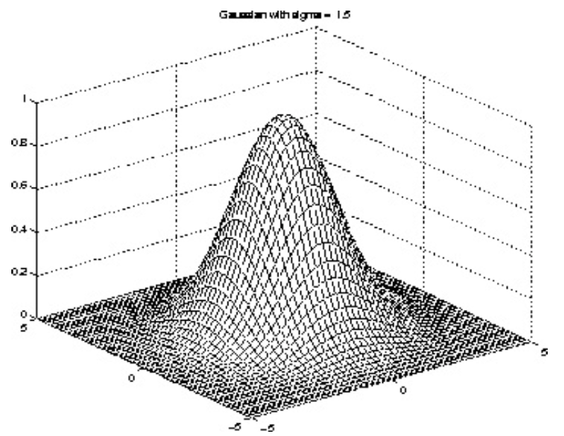
Fig. 97 Gaussian kernels
Polynomial kernel
\[ k\left(\boldsymbol{x}_{1}, \boldsymbol{x}_{2}\right)=\left(1+\boldsymbol{x}_{1}^{\top} \boldsymbol{x}_{2}\right)^{p} \]where the polynomial degree \(p\) is a tuning parameter. \(p=2\) is common.
Pros and Cos
Pros
Kernel PCA can do out-of-sample projection, PCA cannot
Kernel PCA works well when
Cons
Kernel PCA works bad when the data lies a special manifold
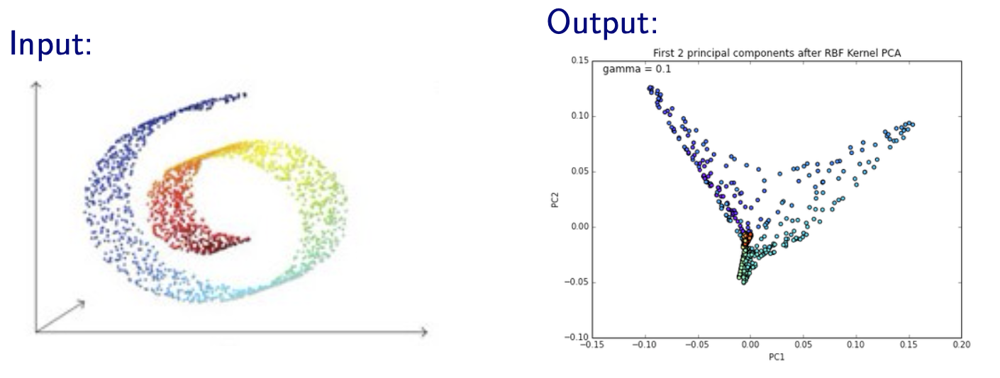
Fig. 100 Kernel PCA with RBF kernel on a Swiss roll manifold [Livescu 2021]
Computationally expensive to compute the \(n \times n\) pairwise kernel values in \(\boldsymbol{K}\) when \(n\) is large. Remedies include
use subset of the entire data set
use kernel approximation techniques
approximate \(\boldsymbol{K} \approx \boldsymbol{F}^\top \boldsymbol{F}\) where \(\boldsymbol{F} \in \mathbb{R} ^{m \times n}, k \ll m \ll n\). The value of \(m\) should be as large as you can handle.
for RBF kernels, there is one remarkable good approximation (due to Fourier transform properties) called random Fourier features (Rahimi & Recht 2008), which replaces each data point \(\boldsymbol{x}_i\) with
\[ \left[\cos \left(\boldsymbol{w}_{1}^{\top} \boldsymbol{x}_{i}+b_{1}\right) \ldots \cos \left(\boldsymbol{w}_{m}^{\top} \boldsymbol{x}_{i}+b_{m}\right)\right]^{\top}=\boldsymbol{f} _{i} \]where
\[\begin{split} \begin{aligned} b_{1}, \ldots, b_{m} & \sim \operatorname{Unif}[0,2 \pi] \\ \boldsymbol{w}_{1}, \ldots, \boldsymbol{w}_{m} & \sim \mathcal{N}\left(0, \frac{2}{\sigma^{2}} \boldsymbol{I}_d \right) \end{aligned} \end{split}\]
just don’t use kernel methods if computation is an issue
Relation to
Standard PCA
Clearly, kernel PCA with linear kernel \(k(\boldsymbol{x} , \boldsymbol{y} ) = \boldsymbol{x} ^\top \boldsymbol{y}\) is equivalent to a standard PCA. That is, they give the same projection.
Derivation
From the analysis above we know that the kernel PCA with linear kernel gives projection of \(\boldsymbol{x}\) as
where \(\boldsymbol{A}_{n \times k}\) is the matrix that stores \(\alpha_{ij}\). Then it remains to prove that \(\boldsymbol{A} ^\top \boldsymbol{X} = \boldsymbol{U} ^\top\) where \(\boldsymbol{U}\) is the projection matrix in conventional PCA: \(\boldsymbol{z} = \boldsymbol{U} ^\top \boldsymbol{x}\). where \(\boldsymbol{A}_{n \times k}\) is the matrix that stores \(\alpha_{ij}\).
Note that in kernel PCA, \(\boldsymbol{\alpha}_j\) are the eigenvectors of the kernel matrix \(\boldsymbol{K}\) since
If we use linear kernel, then \(\boldsymbol{K} = \boldsymbol{X} \boldsymbol{X} ^\top\) and the above relation becomes
Hence, the matrix \(\boldsymbol{A}\) contains the first \(k\) eigenvectors of the Gram matrix \(\boldsymbol{X} \boldsymbol{X} ^\top\).
Now we consider conventional PCA. The projection in \(\mathbb{R} ^k\) is given by
where \(\boldsymbol{U} _{n \times k}\) contains the first \(k\) eigenvectors of the matrix \(\boldsymbol{X} ^\top \boldsymbol{X}\).
Let the singular value decomposition of \(\boldsymbol{X}\) be
The EAD of \(\boldsymbol{X} ^\top \boldsymbol{X}\) is
\[\boldsymbol{X} ^\top \boldsymbol{X} = \boldsymbol{U} \boldsymbol{\Sigma} ^\top \boldsymbol{\Sigma} \boldsymbol{U} = \boldsymbol{U} \boldsymbol{D} \boldsymbol{U}\]where the diagonal entries in \(\boldsymbol{D}\) are the squared singular values \(\sigma^2 _j\) for \(j=1,\ldots, d\).
The EAD for the Gram matrix \(\boldsymbol{G}\)
\[ \boldsymbol{G}_{n \times n}=\boldsymbol{X} \boldsymbol{X}^{\top}=\boldsymbol{A} \boldsymbol{\Sigma} \boldsymbol{\Sigma}^{\top} \boldsymbol{A}^{\top}=\boldsymbol{A} \boldsymbol{\Lambda} \boldsymbol{A}^{\top}=\boldsymbol{A}_{[: d]} \boldsymbol{D} \boldsymbol{A}_{[: d]}^{\top} \]where
\[\begin{split} \boldsymbol{\Lambda}_{n \times n}=\left[\begin{array}{cc} \boldsymbol{D}_{d \times d} & \mathbf{0} \\ \mathbf{0} & \mathbf{0}_{(n-d) \times(n-d)} \end{array}\right] \end{split}\]
Let \(\boldsymbol{a} _j\) be an eigenvector of \(\boldsymbol{G}\) with eigenvalue \(\sigma^2 _j\). Pre-multiplying \(\boldsymbol{G} \boldsymbol{a}_j = \sigma^2 _j \boldsymbol{a} _j\) by \(\boldsymbol{X} ^\top\) yields
Hence, we found that \(\boldsymbol{X} ^\top \boldsymbol{a} _j\) is an eigenvector of \(\boldsymbol{X} ^\top \boldsymbol{X}\) with eigenvalue \(\sigma^2 _j\), denoted \(\boldsymbol{u} _j\),
That is, there is a one-one correspondence between the first \(d\) eigenvectors of \(\boldsymbol{G}\) and those of \(\boldsymbol{X} ^\top \boldsymbol{X}\). More specifically, we have,
which completes the proof.
\(\square\)
Graph-based Spectral Methods
Both are motivates as extensions of MDS and involves a \(n \times n\) matrix.
We can view kernel in kernel PCA as the edge weights in graph-based spectral methods. But the main difference is that in kernel PCA we compute the kernel value of every pair of data points (computationally demanding), but in graph-based spectral methods we only compute weights between points that are neighbors, charactrized by an integer \(k\) or distance \(\epsilon\).
Neural Networks
Kernel PCA can be viewed as a neural network of one single layer with certain constraints.
Let
\(k(\boldsymbol{x}, \boldsymbol{w} )\) be a kernel node parameterized by \(\boldsymbol{w}\) and output the kernel value.
\(w_{ij}\) be the weight of the edge from the \(i\)-th input node to the \(j\)-th hidden node
\(v_{ij}\) be the weight of the edge from the \(i\)-th hidden node to the \(j\)-th output node
Recall our objective is to find \(\boldsymbol{\alpha}_1, \boldsymbol{\alpha} _2, \ldots\) such that the \(j\)-th entry in the embedding is
So the neural network can be designed as
Input layer:
\(d\) nodes, which represent \(\boldsymbol{x} \in \mathbb{R} ^d\)
Kernel layer:
\(n\) kernel nodes, where the \(j\)-th node represents \(k(\boldsymbol{x}, \boldsymbol{x}_i)\)
Fixed weights where \(w_{ij}=1\)
The activation function is simply the identity function
Hidden layer
\(k\) nodes, which represent \(\boldsymbol{z} \in \mathbb{R} ^k\)
Weights \(v_{ij} = \alpha_{ij}\)
The activation function is simply the identity function
Output layer
\(n\) nodes, which represents reconstruction of kernel layer (similar to PCA as autoencoders)
Weights \(\alpha_{ji}\)
The activation function is simply the identity function
Loss: reconstruction loss
In short, we transform the input from \(n\times d\) data matrix \(\boldsymbol{X}\) to \(n\times n\) kernel matrix \(\boldsymbol{K}\), and run PCA. In this way, the learned weights \(\boldsymbol{A}\) are the eigenvectors of \(\boldsymbol{K} ^{\top} \boldsymbol{K}\) (analogous to \(\boldsymbol{X} ^{\top} \boldsymbol{X}\) in PCA), which are the same as \(\boldsymbol{K}\), i.e. what we want for.
Sparse PCA
Recall that \(Z\) is a linear combination of the variables \(X_j\). The original optimization problem is
If we want to impose the number of non-zero coefficient \(a_i\), we can add constraint \(\left\| \boldsymbol{a} \right\| _0 \le k\).
Hui ZOU, Trevor HASTIE, and Robert TIBSHIRANI, 2006
Eigen-space Approach
The problem can be formulated as
Often \(k \ll p\) is desired when \(p\) is large.
Similar to sequential approach in PCA, after obtaining the first principal component \(\boldsymbol{\beta} _1\), we define
and the second sparse principal components can be found by solving the problem
However, unlike the original principal components \(\boldsymbol{a} _i\)’s, the \(\boldsymbol{\beta} _i\)’s are not necessarily orthogonal or uncorrelated to each other without imposing further conditions. In addition, solving this optimization problem turns out to be a very computationally demanding process.
Penalized Regression Approach
One of the alternative approaches for sparse PCA is to devise PCA in a regression setting, then utilize the shrinkage method in linear regression.
Consider the \(i\)-th principal direction \(\boldsymbol{v}_i\) and the corresponding score \(\boldsymbol{z}_i = \boldsymbol{X} \boldsymbol{v}_i\). Now we want a sparse principal direction \(\boldsymbol{\beta}\), but keep the new score \(\boldsymbol{X} \boldsymbol{\beta}\) as close to \(\boldsymbol{z}_i\) as possible. The problem can be formulated as a penalized regression
If we use Ridge regression, then it can be shown that the sparse optimizer \(\boldsymbol{\beta}_{\text{ridge} }\) is parallel to the principal direction \(\boldsymbol{v}_i\):
Derivation
Consider SVD \(\boldsymbol{X} = \boldsymbol{U} \boldsymbol{D} \boldsymbol{V} ^{\top}\), then \(\boldsymbol{X} ^{\top} \boldsymbol{X} = \boldsymbol{V} \boldsymbol{D} ^2 \boldsymbol{V} ^{\top}\),
Hence the loadings are scaled down (attenuated), but still non-zero. We can continue to add \(L_1\) norm. The problem becomes
A larger \(\lambda_1\) will give fewer non-zero component of \(\hat{\boldsymbol{\beta}}\). The estimated coefficients would be an approximation of the principal direction \(\boldsymbol{v} _i\)
where only a few components in \(\hat{\boldsymbol{\beta}}\) is non-zero.
Implementation in R with function spca
In R function spca in library elasticnet, there are many options
type=predictor: use data matrix as inputGram: use covariance matrix or correlation matrix as input
sparse='varnum', para=c(nnz_1, nnz_2): To find sparse loadings, use number of non-zero entries as criteria \(\left\| \boldsymbol{\beta}_i\right\|_0 \le \texttt{nnz_i}\). The numbers are specified inpara.sparse='penalty', para=c(norm_1, norm_2): To find sparse loadings, use the 1-norm of loadings as criteria \(\left\| \boldsymbol{\beta}_i\right\|_1 \le \texttt{norm_i}\). The values of norms are specified inpara.