Geometry
Hyperplanes and Half-spaces
Hyperplanes
For \(\boldsymbol{x} \in \mathbb{R} ^n\), the equation \(\boldsymbol{a} ^\top \boldsymbol{x} = b\) defines a hyperplane \(H\) in \(\mathbb{R} ^n\),
where
\(\boldsymbol{a}\) is a normal vector of that hyperplane, meaning that it is orthogonal to the hyperplane, i.e. it is orthogonal to any vector on the hyperplane. Specifically, let \(\boldsymbol{x} _1, \boldsymbol{x} _2\) be two points on the hyperplane, then \(\boldsymbol{x} _1 - \boldsymbol{x} _2\) is a vector on the hyperplane, and hence \(\boldsymbol{a} ^{\top} (\boldsymbol{x}_1 - \boldsymbol{x}_2) = 0\) for all \(\boldsymbol{x} _1, \boldsymbol{x} _2 \in H\).
\(b\) is the distance from the origin to this hyperplane.
The distance from a point \(\boldsymbol{y}\) to this hyperplane is
note that the distance is always positive.
Derivation
For any two points with coordinates \(\boldsymbol{x}_1, \boldsymbol{x}_2\) on the hyperplane we have
Hence,
which implies that the vector \(\boldsymbol{a}\) is orthogonal to the hyperplane.
The distance from an arbitrary point \(\boldsymbol{y}\) to the hyperplane can be formulated as
where \(\frac{\boldsymbol{a}}{\left\Vert \boldsymbol{a} \right\Vert }\) is a unit vector orthogonal to the hyperplane and \(\boldsymbol{y} - \boldsymbol{x}\) is a vector pointing from point \(\boldsymbol{x}\) (on the hyperplane) to point \(\boldsymbol{y}\). The absolute value of this cross product is the length of the projection of vector \(\boldsymbol{y} - \boldsymbol{x}\) onto the direction of \(\boldsymbol{a}\).
Substituting \(\boldsymbol{a} ^\top \boldsymbol{x} = b\) to this equation gives
Half-spaces
A half-space is either of the two parts into which a hyperplane \((\boldsymbol{a} ^\top \boldsymbol{x} = b)\) divides an affine space.
A strict linear inequality specifies an open half-space:
A non-strict one specifies a closed half-space:
A half-space is a convex set.
Polytopes
Let’s first review some basics.
A polygon (多边形) is a 2-dimensional polytope
A polyhedron (多面体) is a 3-dimensional polytope.
Then, a polytope (多胞体) is a generalization in any number of dimensions. It a geometric object with flat sides. Flat sides mean that the sides of a (k+1)-polytope consist of k-polytopes that may have (k−1)-polytopes in common. For instance, the sides of a polyhedron consist of polygons that may have 1-polytope (dion) in common.
Properties
Convex: A polytope can be convex. For instance, intersection of a set of half-spaces.
Bounded: A polytope is bounded if there is a ball of finite radius that contains it.
- Definition (full-dimensional)
A polyhedron \(P \in \mathbb{R} ^n\) is full-dimensional if it has positive volume. Equivalently,
if it has \(n+1\) affinely independent points
if it contains a ball of positive radius
Ellipsoids
An ellipsoid is a generalization of an ellipse into any number of dimensions.
In 3-d case, the implicit equation of an ellipsoid has the standard form
Fig. 6 Sphere (\(a = b = c\), top), Spheroid (\(a = b \ne c\), bottom left), Tri-axial ellipsoid (\(a,b,c\) all different, bottom right)
Characterization
Formally, a set \(E\) of vectors in \(\mathbb{R} ^n\) of the form
where \(\boldsymbol{D}\) is an \(n\times n\) positive definite matrix, is called an ellipsoid with center \(\boldsymbol{z} \in \mathbb{R} ^n\).
Other formulation: \(E(\boldsymbol{b} , \boldsymbol{A})=\left\{\boldsymbol{x} \in \mathbb{R} ^2:\|\boldsymbol{A} \boldsymbol{x} -\boldsymbol{b} \|_{2} \leq 1\right\}\) where \(\boldsymbol{A}\) is p.d. The volume of \(E\) is proportional to \(\operatorname{det} (\boldsymbol{A} ^{-1} )\).
Relation between \((\boldsymbol{z} ,\boldsymbol{D})\) and \((\boldsymbol{b}, \boldsymbol{A})\):
Hence, the relation is \(\boldsymbol{z} = \boldsymbol{A} ^{-1} \boldsymbol{b}\) and \(\boldsymbol{D} = (\boldsymbol{A} ^{\top} \boldsymbol{A} ) ^{-1}\), or \(\boldsymbol{b} = \boldsymbol{A} \boldsymbol{z}\) and \(\boldsymbol{A} = \boldsymbol{D} ^{-1/2}\). Hence \(\operatorname{vol} (E) \propto \operatorname{det} (\boldsymbol{D} ^{1/2})\), or \(\operatorname{det} (\boldsymbol{D} ) \propto \operatorname{vol}(E)^2\). We use many properties of positive definite matrices, see the relevant section.
Ball
For any \(r >0\), the ellipsoid
is called a ball centered at \(\boldsymbol{z}\) of radius \(r\).
Cones
Normal Cones
The normal cone of a convex set \(S\) at a point \(\boldsymbol{x} \in S\) is defined as
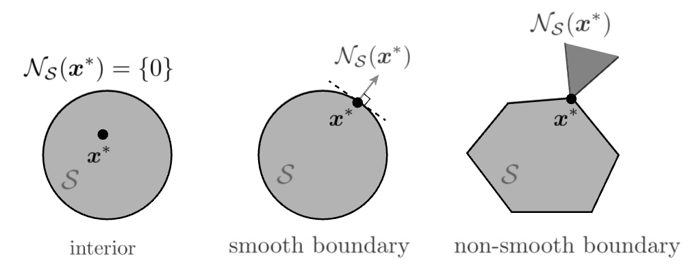
Fig. 7 Normal cones [Friedlander and Joshi]
For instance,
For an affine set
\[S = \left\{ \boldsymbol{x} \mid \boldsymbol{c} _i ^{\top} \boldsymbol{x} = b_i, i = 1, 2, \ldots, m \right\}\]The normal cone is just a linear combination of all vectors perpendicular to the hyperplanes
\[N_S (\boldsymbol{x}) = \left\{ \sum_{i=1}^m \lambda_i \boldsymbol{c} _i \mid \lambda _i \in \mathbb{R} \right\}\]It easy to see that \(\boldsymbol{c} _i ^{\top} (\boldsymbol{y} - \boldsymbol{x} ) = 0\) for all \(i\) and \(\boldsymbol{y} \in S\). If we write \(\boldsymbol{C} \boldsymbol{x} = \boldsymbol{b}\), then the normal cone is the linear combination of rows of \(\boldsymbol{C}\), i.e. \(\operatorname{range} (\boldsymbol{C} ^{\top})\).
For a set of points with non-negative coordinates
\[S = \left\{ \boldsymbol{x} \in \mathbb{R} ^n \mid x_j \ge 0, \forall j = 1, 2, \ldots, n \right\}\]For a point \(\boldsymbol{x} \in S\), define an active set \(A(\boldsymbol{x}) = \left\{ j \mid x_j = 0 \right\}\) that consists of the indices of zero coordinates of \(\boldsymbol{x}\). The normal cone of \(S\) at \(\boldsymbol{x}\) is
\[N_S (\boldsymbol{x} ) = \left\{ - \sum_{j \in A(\boldsymbol{x})} \mu_j \boldsymbol{e} _j \mid \mu_{j} \ge 0\right\}\]where \(\boldsymbol{e}_j\) are canonical vectors. The set can also be expressed as
\[N_S (\boldsymbol{x} ) = \left\{ - \sum_{j=1}^n \mu_j \boldsymbol{e} _j \mid \mu_{j} \ge 0, \sum_{j=1}^n\mu_j x_j =0\right\}\]which states that \(\mu_j = 0\) as long as \(x_j \ne 0\). In matrix form, we can write it as
\[N_S (\boldsymbol{x} ) = \left\{ - \boldsymbol{\mu} \mid \boldsymbol{\mu} \ge 0, \langle \boldsymbol{\mu} , \boldsymbol{x} \rangle > 0\right\}\]More generally, combining them together,
\[S = \left\{ \boldsymbol{x} \in \mathbb{R} ^n\mid \boldsymbol{c} _i ^{\top} \boldsymbol{x} = b_i, x_j \ge 0 \ \forall i \in [m], j \in [n]\right\}\]The normal cone is
\[N_S (\boldsymbol{x} ) = \left\{ \sum_{i=1}^m \lambda_i \boldsymbol{c} _i - \boldsymbol{\mu} \mid \lambda _i \in \mathbb{R}, \boldsymbol{\mu} \ge 0, \langle \boldsymbol{\mu} , \boldsymbol{x} \rangle > 0\right\}\]