Sampling¶

In this section we introduce some some sampling methods for various problem settings. Suppose we generate a sample $\left\{ x_1, x_2, \ldots, x_n \right\}$ from some distribution $p(x)$.

If the exact functional form of $p(x)$ is unknown or hard to obtain, but we know some function $f(x)$ that is proportional to $p(x)$ up to some normalizing constant, then we can use $f(x)$ to obtain the sample. Some methods include

Rejection sampling
Markov Chain Monte Carlo
- Metropolis Hastings

For multivariate distributions, e.g. $d=2$, if we want to generate a sample $\left\{ (x_1, y_1), \ldots, (x_n, y_n) \right\}$ from unknown $p(x,y)$, and $f(x \vert y )\propto p(x\vert y)$ and $f(y \vert x )\propto p(x\vert y)$ are known, then we can use $f(x \vert y)$ and $f(y \vert x)$ to obtain the sample. Gibbs sampling solve this problem setting.

Estimation of Mean and Total¶

Setup

a population $U = \left\{ 1, \ldots, N_u \right\}$ of $N_u$ units, e.g. people, animals
a value $y_i$ for each $i \in U$, e.g. height, age
$\tau = \sum_{i \in U} y_i$ is the total, and $\mu = \frac{\tau}{N_u}$ is the average, of $y$’s in the population
$S = \left\{ i_1, \ldots, i_n \right\}$ is a sample of $n$ units from $U$, and we can observe $y_i$ for each $i \in S$.

Estimation of population total $\tau$ or average $\mu$ from a random sample is an ubiquitous task.

Equal Probability Sampling¶

With Replacement¶

Consider a sample $S$ uniformly from $U$ with replacement, then we have unbiased estimates

\[ \hat{\mu} = \frac{1}{n} \sum_{i \in S} y_i \quad \hat{\tau} = N_u \bar{y} \]

with variance

\[ \operatorname{Var}\left( \hat{\mu} \right) = \frac{\sigma^2}{n} \quad \operatorname{Var}\left( \hat{\tau} \right) = \frac{N_u^2\sigma^2}{n} \]

where $\sigma^2$ is the population variance, which can be estimates by $s^2 = \frac{1}{n-1} \sum_{i \in S} (y_i - \bar{y})^2$.

Without Replacement¶

Now consider sampling without replacement. The inclusion probability of unit $i$ in a sample of size $n$ is

\[ \pi_i = \frac{\binom{N_u - 1}{n-1} }{\binom{N_u}{n} } = \frac{n}{N_u} \]

Similarly, let $\pi_{ij}$ be the probability that units $i$ and $j$ are both in the sample $S$, we have

\[ \pi_{ij} = \frac{n(n-1)}{N_u(N_u - 1) } \]

The unbiased estimates of the mean and total have the same form

\[ \hat{\tau}_\pi = N_u \bar{y} \quad \hat{\mu}_\pi = \bar{y} \]

but smaller variance

\[ \operatorname{Var}\left( \hat{\mu}_\pi \right) = \frac{N_u - n}{N_u } \frac{ \sigma^2 }{n} < \frac{\sigma^2 }{n} \quad \operatorname{Var}\left( \hat{\tau}_\pi \right) = \frac{N_u (N_u - n) \sigma^2 }{n} < \frac{N_u ^2 \sigma^2 }{n} \]

Unequal Probability Sampling¶

In many situations, some units are more likely than others to be included in a sample, either by design or by accident, e.g. interviewing people on a street, locating homeless vs homeowners, etc. Sampling under designs of this sort is called unequal probability sampling.

In this setting, the sample mean is a biased estimator for $\mu$. The Horvitz-Thompson estimator remedies this problem. Note that the Horvitz-Thompson estimator does not depend on the number of times a unit may be selected. Each distinct unit of the sample is utilized only once. We first consider sampling without replacement such that all units in $S$ is distinct.

Horvitz-Thompson Estimate¶

Suppose that each unit $i \in U$ has probability $\pi_i$ of being included in a sample $S$ of size $n$. The Horvitz-Thompson estimate of $\tau$ and $\mu$ is

\[ \hat{\tau}_\pi = \sum_{i \in S} \frac{y_i}{\pi_i} \quad \hat{\mu}_\pi = \frac{1}{N_u} \hat{\tau}_\pi \]

the estimator $\hat{\tau}_\pi$ is unbiased since

\[ \mathbb{E}\left(\hat{\tau}_{\pi}\right)=\mathbb{E}\left(\sum_{i \in S} \frac{y_{i}}{\pi_{i}} \right)=\mathbb{E}\left(\sum_{i \in {U}}\frac{y_{i}}{\pi_{i}} Z_i\right)=\sum_{i \in {U}} \frac{y_{i}}{\pi_{i}} \mathbb{E}\left(Z_{i}\right) = \tau \]

where $Z_i = 1$ if $i \in S$ and zero otherwise, hence $\mathbb{E}\left( Z_i \right) = \mathbb{P}\left( Z_i = 1 \right) = \pi_i$.

To find the variance of this estimator, use the indicator variable approach, we obtain

\[\begin{split}\begin{aligned} \mathbb{V}\left(\hat{\tau}_{\pi}\right) &= \operatorname{Cov} \left(\sum_{i \in {U}}\frac{y_{i}}{\pi_{i}} Z_i, \sum_{i \in {U}}\frac{y_{i}}{\pi_{i}} Z_i\right) \\ &= \sum_{i\in U}\left(\frac{1-\pi_{i}}{\pi_{i}}\right) y_{i}^{2}+\sum_{i\in U}\sum_{j \neq i}\left(\frac{\pi_{i j}-\pi_{i} \pi_{j}}{\pi_{i} \pi_{j}}\right) y_{i} y_{j} \\ &=\sum_{i \in U} \sum_{j \in U} y_{i} y_{j}\left(\frac{\pi_{i j}}{\pi_{i} \pi_{j}}-1\right) \quad \text{$\pi_{ij} = \pi_i$ when $i = j$.} \end{aligned}\end{split}\]

An unbiased estimator for this is

\[\begin{split}\begin{aligned} \widehat{\mathbb{V}}\left(\hat{\tau}_{\pi}\right) &= \sum_{i\in S}\left(\frac{1-\pi_{i}}{\pi_{i}^{2}}\right) y_{i}^{2}+\sum_{i\in S} \sum_{j \neq i}\left(\frac{\pi_{i j}-\pi_{i} \pi_{j}}{\pi_{i} \pi_{j}}\right) \frac{1}{\pi_{i j}} y_{i} y_{j} \\ &=\sum_{i \in S} \sum_{j \in S} y_{i} y_{j}\left(\frac{1}{\pi_{i} \pi_{j}}-\frac{1}{\pi_{i j}}\right) \end{aligned}\end{split}\]

assuming $\pi_{ij} > 0$ for all pairs $(i, j)$. In particular, if the inclusion of units $i$ and $j$ are independent, then $\pi_{ij} = \pi_i \pi_j$, and only diagonal term $(i=j)$ remains in the above two quantities.

An approximate $(1-\alpha)$ 100% confidence interval for $\tau$ is

\[ \hat{\tau}_{\pi} \pm t_{\alpha / 2} \sqrt{ \hat{\mathbb{V}}\left(\hat{\tau}_{\pi}\right)} \]

The two analogous quantities for estimator $\hat{\mu}_\pi$ are

\[ \mathbb{V}\left(\hat{\mu}_{\pi}\right)=\frac{1}{N_u^2} \mathbb{V}\left(\hat{\tau}_{\pi}\right) \quad \mathbb{V}\left(\hat{\mu}_{\pi}\right)=\frac{1}{N_u^2} \widehat{\mathbb{V}}\left(\hat{\tau}_{\pi}\right) \]

With Replacement¶

Now we consider sampling with replacement. We first obtain a sample $S$ of size $n$, then find a set $S^*$ of distinct units from $S$, and use $S^*$ to compute the Horvitz-Thompson estimates.

Let $p_i$ be the probability of being selected in each of the $n$ times for $i \in U$. It is easy to see that the inclusion probability in $S^*$ (or equivalently, sample $S$) are

\[\begin{split}\begin{aligned} \pi_i &= 1 - (1-p_i)^n\\ \pi_{ij} & = \mathbb{P}\left( i \in S \right) + \mathbb{P}\left( j \in S \right) - \mathbb{P}\left( i,j \in S \right) \\ &= \pi_i + \pi_j - [1 - (1-p_i - p_j)^n] \end{aligned}\end{split}\]

Horvitz-Thompson estimators can be computed with these values.

If $p_i$ is directly proportional to the values $c_i$ of some characteristic of $i$, i.e., $p_i = \frac{c_i}{\sum c_i}$ we call this probability proportional to size (PPS) sampling. For instance, households might be selected for a marketing survey by drawing names from a database, in which case those households with more members in the database have a larger chance of being included.

Estimation of Group Size and Species¶

Group Size¶

The estimation of group total $\tau$ above usually involve $N_u$, but often $N_u$ is unknown, e.g. populations of endangered animal species. One method to estimate $N_u$ is the class of capture-recapture estimators. The simplest version involves two stages

Select a simple random sample $S_1$ of size $n_1$ without replacement, mark all units in $S_1$, and return then to the population
Select a simple random sample $S_2$ of size $n_2$ without replacement, the value

\[ \hat{N}_u^{(c/r)} = \frac{n_2}{m} n_1 \]

is then used as an estimate of $N_u$, where $m = \left\vert S_1 \cap S_2 \right\vert$ is the number of marked units in $S_2$. An estimator of the variance is

\[ \widehat{V}\left(\hat{N}_{u}^{(c / r)}\right)=\frac{n_{1} n_{2}\left(n_{1}-m\right)\left(n_{2}-m\right)}{m^{3}} \]

If $n_1$ and $n_2$ are fixed, then $m$ follows a hypergeometric distribution, and the integer part of $\hat{N}_u^{(c/r)}$ corresponds to MLE of $N_u$.

Group Species¶

Aka species problem. Suppose there $N_s$ number of species in the forest, how to estimate $N_s$? Similar problems include how many words did Shakespeare know based on his published works, and how many kinds of ancient coins minted by a society based on archaeological finds.

It is possible that there are an arbitrary number of species in the population in arbitrarily small proportions. This fact allows for the species problem to potentially be quite ill-posed.

One nonparametric estimator called coverage estimator of $N_s$ adjusts the number of observed species $n_{obs}$ upward by a certain factor (??)

\[ \hat{N}_s^{cov} = \frac{n_s ^{obs}}{\hat{c}} \quad \text{where} \quad \hat{c} = 1 - \frac{x_1}{n} \]

where $x_1$ is the number of species observed only once in the sample of size $n$. The factor $\hat{c}$ is an estimate of the coverage $c$ of the sample: the fraction of population corresponding to species observed at least once.

Pros

has asymptotic behavior quite close to that of MLE
easier to compute than MLE

Cons

suffer from significant bias and large variance in small samples

Monte Carlo¶

Given a random variable $X$ with PDF $f$, sometimes we need to compute the expectation of $g(X)$:

\[ \mathbb{E}\left( g(X) \right) = \int g(x)f(x) \mathrm{~d}x \]

When computationally tractable, closed form expressions are not available for this purpose, and numerical integration is infeasible. For instance, Monte Carlo method generate random draws $x_1, \ldots, x_n$ of $X$ from $f$, and compute the stochastic approximation

\[ \widehat{\mathbb{E}}(g(X))=\frac{1}{n} \sum_{i=1}^{n} g\left(x_{i}\right) \]

Sometimes it is hard to generate random draws from $f$. If we can sample from $h$ where $w(x) = \frac{f(x)}{h(x)}$, then by re-arrangement we have

\[ \mathbb{E}(g(X))= \frac{\int g(x) w(x) h(x) \mathrm{~d} x }{\int w(x) h(x) \mathrm{~d} x} \]

Hence the approximation is

\[ \widehat{\mathbb{E}}_{h}(g(X)) = \frac{(1 / n) \sum_{i=1}^{n} w\left(x_{i}\right) g\left(x_{i}\right)}{(1 / n) \sum_{i=1}^{n} w\left(x_{i}\right)} \]

Rejection Sampling¶

Markov Chain Monte Carlo¶

General Setting¶

Metropolis Hastings¶

MH is a particular case of MCMC.

Gibbs Sampling¶

Others¶

Finite Population Sampling

Poisson Sampling¶

Bernoulli Sampling¶

Exercise¶

Sampling from a Triangle¶

Tags: TwoSigma, Quant, 20Q4

How to generate uniformly distributed points in a triangle in a $xy$-plane, given the coordinates of the three vertices? Suppose that you have a generator that can generate uniformly distributed random values over the interval $[0,1]$ and you can use it twice.

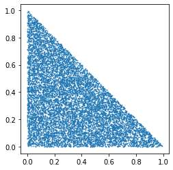
We can first start from a special case and then generalize it: what if the three coordinates are $(0,0), (0,1), (1,0)$? Call this triangle the basic triangle.

We can draw a random point $(x, y)$ from the square with vertices $(0,0), (0,1), (1,1), (1,0)$, using twice the random generator. If the point is inside the basic triangle, which is identified by $x+y<1$, then we keep it, otherwise $x+y>1$ we keep its symmetric point $(1-x, 1-y)$ which is inside the basic triangle. The sampling process is implemented in the below python script.

import numpy as np
import matplotlib.pyplot as plt

def sample_basic_triangle(n):
    points = np.random.rand(n,2)
    inside = points[:,0] + points[:,1] < 1
    sample = np.where(inside.reshape(n,1), points, 1-points)
    return sample

points = sample_basic_triangle(10000)
plt.scatter(points[:,0], points[:,1], s=0.5)
plt.gca().set_aspect('equal')
plt.show()

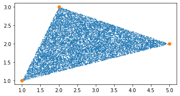
Then, for any triangle $ABC$, given the $xy$-coordinates of three vertices $A, B, C$, we can choose a reference point, say $A$, and two edges vectors $AB$ and $AC$. Any random point inside the triangle $ABD$ can be expressed as a linear combination of the two edge vectors $P = v \cdot AB + w \cdot AC$, where $v$ and $w$ are from independent uniform distribution. Modifying the above algorithm we have the required results.

def sample_any_triangle(vers, n):
    points = np.random.rand(n,2)
    inside = points[:,0] + points[:,1] < 1
    ref = vers[0]
    e1 = vers[1] - ref
    e2 = vers[2] - ref
    scale = np.where(inside.reshape(n,1), points, 1-points)
    sample = scale @ np.vstack((e1,e2)) + ref
    return sample

vers = np.asarray([[1,1], [5,2], [2,3]]) # vertices coordinates
points = sample_any_triangle(vers, 10000)
plt.scatter(points[:,0], points[:,1], s=0.5)
plt.scatter(vers[:,0], vers[:,1])
plt.gca().set_aspect('equal')
plt.show()

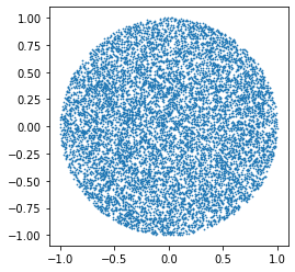
Sample from a Disk¶

How to uniformly sample points inside a disk? Can you take advantage of the above method of sampling from a triangle?

n = 10000
vers = np.asarray([[0,0], [0,1], [0,1]])
points = sample_any_triangle(vers, n)
theta = np.random.rand(n)*2*np.pi
Rs = np.array([[np.cos(theta), -np.sin(theta)], [np.sin(theta), np.cos(theta)]]).transpose()
sample = np.array([points[i] @ Rs[i] for i in range(n)])
plt.scatter(sample[:,0], sample[:,1], s=0.5)
plt.gca().set_aspect('equal', adjustable='box')

Data Science Handbook

Sampling¶

Estimation of Mean and Total¶

Equal Probability Sampling¶

With Replacement¶

Without Replacement¶

Unequal Probability Sampling¶

Horvitz-Thompson Estimate¶

With Replacement¶

Estimation of Group Size and Species¶

Group Size¶

Group Species¶

Monte Carlo¶

Rejection Sampling¶

Markov Chain Monte Carlo¶

General Setting¶

Metropolis Hastings¶

Gibbs Sampling¶

Others¶

Poisson Sampling¶

Bernoulli Sampling¶

Exercise¶

Sampling from a Triangle¶

Sample from a Disk¶