Autoencoders¶

Objective¶

An autoencoder is a type of neural networks used to learn efficient data encodings/representations in an unsupervised manner. It is constituted by two main parts:

an encoder $\boldsymbol{\phi} (\cdot)$ that maps the input into the code $\boldsymbol{z} = \boldsymbol{\phi(\boldsymbol{x} )}$, and
a decoder $\boldsymbol{\psi} (\cdot)$} that maps the code $\boldsymbol{z}$ to a reconstruction of the original input $\boldsymbol{x} ^\prime = \boldsymbol{\psi}(\boldsymbol{z})$.

As a result, the output layer has the same number of nodes as the input layer. The structure is shown below

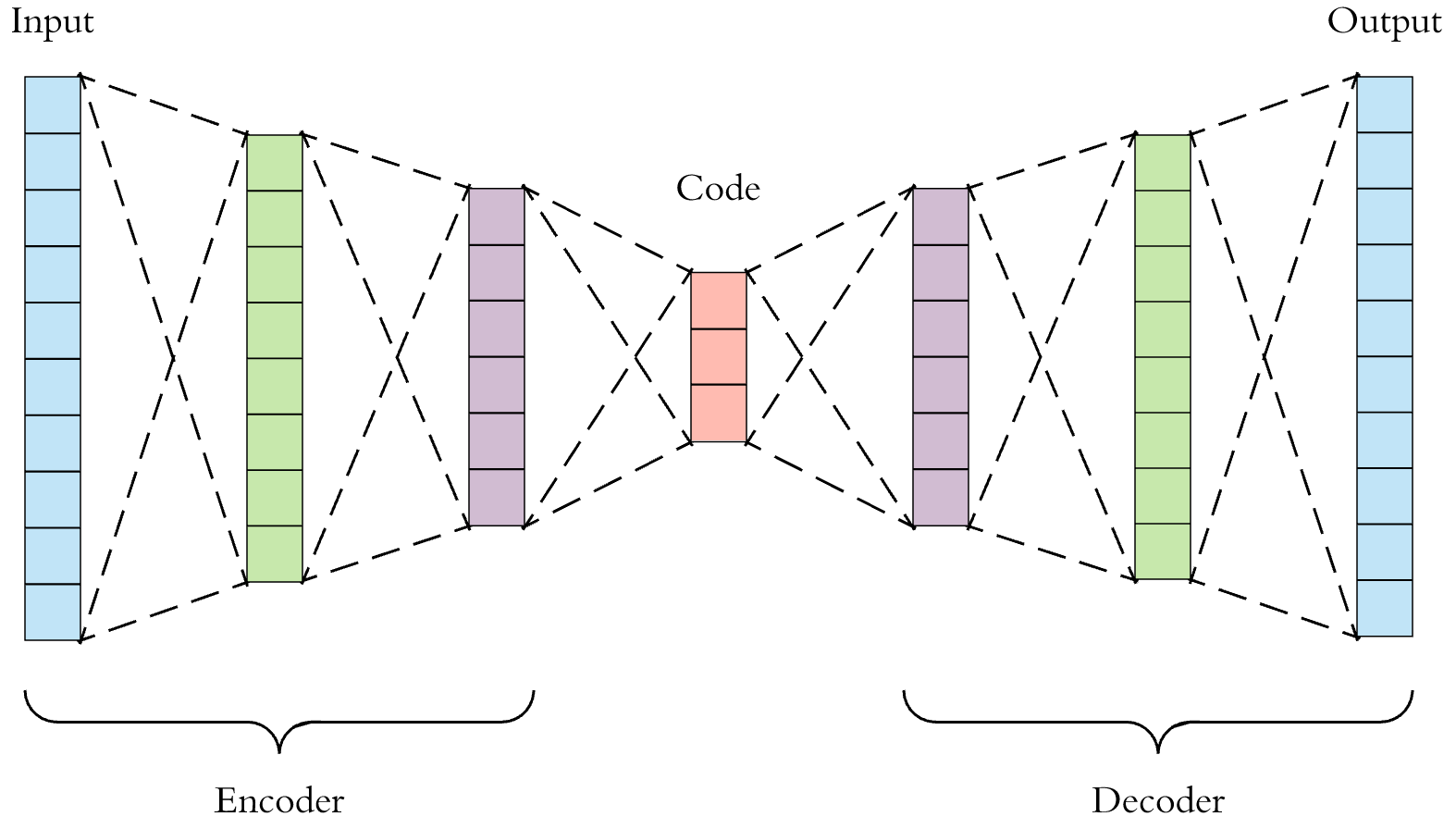
Fig. 166 Structure of Autoencoders¶

The objective is minimizing the difference between the input $\boldsymbol{x}$ and the output $(\boldsymbol{\psi} \circ \boldsymbol{\phi} )\boldsymbol{x}$,

\[\begin{split} \begin{array}{l} \text{encoder}\qquad \boldsymbol{\psi} :\mathcal{X}\rightarrow\mathcal{Z}\\ \text{decoder}\qquad \boldsymbol{\psi} :\mathcal{Z}\rightarrow\mathcal{X}\\ \qquad\qquad \boldsymbol{\phi,\psi} =\underset{\boldsymbol{\phi,\psi} }{\arg\min}\|\boldsymbol{x} -(\boldsymbol{\psi} \circ \boldsymbol{\phi} )\boldsymbol{x} \|^{2} \end{array} \end{split}\]

Example

In the simplest case, given one hidden layer, the encoder stage of an autoencoder takes the input $\boldsymbol{x}\in\mathbb{R}^{d}=\mathcal{X}$ and maps it to code/representation/latent variable $\boldsymbol{z}\in\mathbb{R}^{k}=\mathcal{Z}$.

\[ \boldsymbol{z}=\sigma(\boldsymbol{W}\boldsymbol{x}+\boldsymbol{b}) \]

Like other neural networks, the weights $\boldsymbol{W}$ and biases $\boldsymbol{b}$ are initialized randomly and updated iteratively during training through backpaopagation.

The decoder stage of the antoencoder maps $\boldsymbol{h}$ to the reconstruction $\boldsymbol{x}'$ of the same shape as $\boldsymbol{x}$. $$ \boldsymbol{x}^{\prime}=\sigma^{\prime}\left(\boldsymbol{W}^{\prime}\boldsymbol{z}+\boldsymbol{b}^{\prime}\right) $$

Autoencoders are trained to minimize reconstruction loss

\[ \mathcal{L}\left(\boldsymbol{x},\boldsymbol{x}^{\prime}\right)=\left\Vert \boldsymbol{x}-\boldsymbol{x}^{\prime}\right\Vert ^{2}=\left\Vert \boldsymbol{x}-\sigma^{\prime}\left(\boldsymbol{W}^{\prime}(\sigma(\boldsymbol{W}\boldsymbol{x}+\boldsymbol{b}))+\boldsymbol{b}^{\prime}\right)\right\Vert ^{2} \]

Number of neurons in the code layer

Does the number of neurons in the code layer matters?

Should the feature space ${\displaystyle {\mathcal{Z}}}$ have lower dimensionality than the input space ${\displaystyle {\mathcal{X}}}$, the feature vector ${\displaystyle \boldsymbol{z}=\boldsymbol{\phi} (\boldsymbol{x})}$ can be regarded as a compressed representation of the input $\boldsymbol{x}$. This is the case of undercomplete autoencoders.
If the hidden layers are larger than (overcomplete autoencoders), or equal to, the input layer, or the hidden units are given enough capacity, an autoencoder can potentially learn the identity function and become useless.

However, experimental results have shown that autoencoders might still learn useful features in these cases. In the ideal setting, one should be able to tailor the code dimension and the model capacity on the basis of the complexity of the data distribution to be modeled. One way to do so, is to exploit the model variants known as Regularized Autoencoders.

In general, autoencoders only make sense if we constrain $\boldsymbol{\phi} (\cdot)$ somehow. For instance,

Limit dimensionality of $\boldsymbol{\phi} (\boldsymbol{x})$
Add a penalty to the loss, e.g. to induce sparsity in the learned representation
Denoising autoencoders: Add noise to the input, but try to reproduce the clean input. The autoencoder learn to extract essential information of the input.

View decoder as a distribution

The decoder part can be viewed as representing a distribution $p(\boldsymbol{x} \mid \boldsymbol{z})$ over the encoder input $\boldsymbol{x}$ given the output $\boldsymbol{z} = f(\boldsymbol{x})$, like probabilistic PCA.

If $p(\boldsymbol{x} \mid \boldsymbol{z})$ is, say, a spherical Gaussian with mean $\boldsymbol{\psi}(\boldsymbol{z} )$, then optimizing the likelihood over a training set is equivalent to the usual squared loss.

Other distributions produce different losses.

Variants and Application¶

The most traditional application was dimensionality reduction or feature learning. Several variants exist to the basic model, with the aim of forcing the learned representations of the input to assume useful properties. Examples are the

Regularized autoencoders

Various techniques are applied to prevent autoencoders from learning the identity function and to improve their ability to capture important information and learn richer representations. They are proven effective in learning representations for subsequent classification tasks. Some examples include
- sparse encoders
- denoising encoders
- contractive autoencoders
Variational autoencoders

Recent applications as generative models.

Here we introduce regularized autoencoders. Variational autoencoders are introduced in a separated section.

Sparse Autoencoders¶

Sparse autoencoder may include more hidden units than inputs, but only a small number of them are active at once, determined by the input $\boldsymbol{x}_{i}$. This sparsity constraint forces the model to respond to the unique statistical features of the input data used for training.

The objective include a sparsity penalty term $R(\boldsymbol{z})$ on the code layer $\boldsymbol{z}$.

\[ \mathcal{L}\left(\boldsymbol{x},\boldsymbol{x}^{\prime}\right)+R(\boldsymbol{z}) \]

For instance, we can use L1 or L2 regularization,

\[ \mathcal{L}\left(\boldsymbol{x},\boldsymbol{x}^{\prime}\right)+\lambda\left\Vert \boldsymbol{z}\right\Vert \]

Denoising Autoencoders¶

Instead of using the original input $\boldsymbol{x}$, we add noise and use the corrupted input $\tilde{\boldsymbol{x}}$. Denoising autoencoders take a partially correpted (noised) input $\tilde{\boldsymbol{x}}$ and are trained to recover the original undistorted input. So it’s called denoising. There are two underlying assumptions

Higher level representations are relatively more stable and robust to the corruption of the input
To perform denoising well, the model needs to extract features that capture useful structure in the distribution of the input.

Essentially, we model

\[\begin{split} \begin{aligned} \tilde{\boldsymbol{x}} & \sim q_{D}(\tilde{\boldsymbol{x}}\mid\boldsymbol{x})\\ \boldsymbol{z} & =\phi(\tilde{\boldsymbol{x}})\\ \boldsymbol{x}^{\prime} & =\psi(\boldsymbol{z}) \end{aligned} \end{split}\]

The objective function is still to minimize the reconstruction error

\[ \mathcal{L}\left(\boldsymbol{x},\boldsymbol{x}^{\prime}\right) \]

The corruption process $q_{D}(\tilde{\boldsymbol{x}}\mid\boldsymbol{x})$ might be

Additive isotropic Gaussian noise,
Masking noise: a fraction of the input chosen at random for each example is forced to 0
Salt-and-pepper noise: a fraction of the input chosen at random for each example is set to its minimum or maximum value with uniform probability

Finally, notice that the corruption of the input is performed only during the training phase of the. Once the model has learnt the optimal parameters, in order to extract the representations from the original data, no corruption is added.

Contractive Autoencoders¶

Contractive autoencoder (CAE) adds an explicit regularizer in their objective function that forces the model to learn a function that is robust to slight variations of input values.

This regularizer corresponds to the Frobenius norm of the Jacobian matrix of the encoder activations with respect to the input. Since the penalty is applied to training examples only, this term forces the model to learn useful information about the training distribution. Theobjective function has the following form:

\[ \mathcal{L}\left(\boldsymbol{x},\boldsymbol{x}^{\prime}\right)+\lambda\left\Vert \nabla_{\boldsymbol{x}}\boldsymbol{z}\right\Vert ^{2} \]

The name contractive comes from the fact that CAE is encouraged to map a neighborhood of input points to a smaller neighborhood of output points.

There is a connection between the denoising autoencoder (DAE) and the contractive autoencoder (CAE): in the limit of small Gaussian input noise,

DAE make the reconstruction function resist small but finite-sized perturbations of the input,
CAE make the extracted features resist infinitesimal perturbations of the input.

Data Science Handbook