Linear Models - Diagnosis
No models are perfect. In this section we introduce what happen when our model is misspecified or when some assumptions fail. We will introduce how to diagnose these problems, and corresponding remedies and alternative models, e.g. Lasso, ridge regression, etc.
Special Observations
Outliers
- Definition (Outliers)
There are many ways to define outliers. Observations \(i\) is an outlier
univariate measure: if \(\left\vert x_{ji} - \mu_j \right\vert\) is larger than some threshold, say some multiples of standard deviations of \(X_j\), then the \(j\)-th value of observation \(i\) is an outlier w.r.t. other observations of variable \(X_j\).
multivariate measure: if \(\left\| \boldsymbol{x}_i -\boldsymbol{\mu} \right\|^2\) is larger than some threshold, then \(\boldsymbol{x}_i\) an outlier w.r.t. other data points in \(\boldsymbol{X}\).
if its studentized residual \(\left\vert t_i \right\vert\) is larger than some threshold, say \(t_{n-p}^{(\alpha/2n)}\)
- Solution
If outlier is a mistake (typo) you can drop it (or correct it)
If outlier is valid but unusual, look for robustness – does dropping it change answer?
If it does change answer, report both versions – and argue for the approach you think more appropriate
Leverage Points
- Definition (Leverages and leverage points)
Leverage (score) of an observation \(i\) is defined as \(h_i = \boldsymbol{x}_i ^\top (\boldsymbol{X} ^\top \boldsymbol{X} ) ^{-1} \boldsymbol{x}_i\). It is the \(i\)-th diagonal entry of the projection matrix \(\boldsymbol{H} = \boldsymbol{X} (\boldsymbol{X} ^\top \boldsymbol{X} )^{-1} \boldsymbol{X} ^\top = \boldsymbol{P}_{\operatorname{im} (\boldsymbol{X} )}\).
If \(h_i\) is large than some threshold, say \(2p/n\), then we say \(i\) is a leverage point.
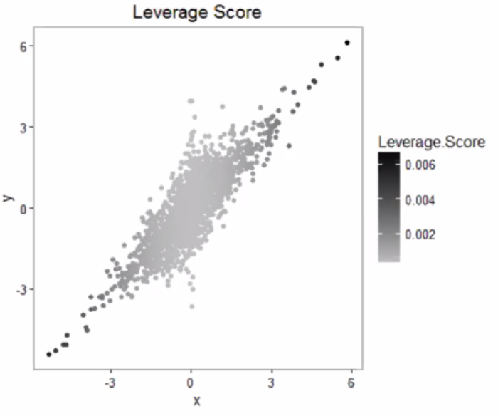
Fig. 63 Leverage scores [Zhang+ 2018]
- Properties
In particular, we have \(0<h_i<1\) and \(\sum_{i=1}^n h_i = p\), or \(\bar{h} = p/n\)
Recall that \(\operatorname{Var}\left( \hat{\boldsymbol{\varepsilon} } \right) = \operatorname{Var}\left( \boldsymbol{y} - \hat{\boldsymbol{y}} \right)= \sigma^2 (\boldsymbol{I} - \boldsymbol{H} )\), so \(\operatorname{Var}\left( \hat{\varepsilon}_i \right) = \sigma^2 (1-h_i)\)
- Definition (Standardized residuals)
Standardized residuals is defined as
\[ r_i = \ \frac{\hat{\varepsilon}_i}{\sigma\sqrt{1- h_i}} \]It is standardized since \(\operatorname{Var}\left( r_i \right) = 1\). But in practice, we don’t know \(\sigma\). So we plug in its estimate \(\hat{\sigma}\).
Influential Points
- Definition (Influential points)
Influential points are data points such that if we remove it, the model changes substantially. It can be quantified by Cook’s distance
\[ D_i = \frac{r_i ^2}{p} \frac{h_i}{1-h_i} \]where \(r_i\) is standardized residual.
Note
A influential point can be close to the fitted line. If we drop it, then there seems no linear relation in the remaining data cloud.
Two or more influential points near each other can mask each other’s influence in a leave-one-out regression. That is, if remove any one of them, then the regression results do not change substantially, but if we remove both of them, then the results change substantially.
Omitting a Variable
Suppose the true model is
And we omit one explanatory variable \(X_j\). Thus, our new design matrix has size \(n \times (p-1)\), denoted by \(\boldsymbol{X}_{-j}\). Without loss of generality, let it be in the last column of the original design matrix, i.e. \(\boldsymbol{X} = \left[ \boldsymbol{X} _{-j} \quad \boldsymbol{x}_j \right]\). The new estimated coefficients vector is denoted by \(\widetilde{\boldsymbol{\beta}}_{-j}\). The coefficient for \(\boldsymbol{x}_j\) in the true model is denoted by \(\beta_j\), and the vector of coefficients for other explanatory variables is denoted by \(\boldsymbol{\beta} _{-j}\). Hence, \(\boldsymbol{\beta} ^\top = \left[ \boldsymbol{\beta} _{-j} \quad \beta_j \right] ^\top\).
We first find the expression of the new estimator \(\hat{\boldsymbol{\beta}}_{-j}\) of the regression where the design matrix is \(\boldsymbol{X} _{-j}\).
The expectation, therefore, is
What is \(\left( \boldsymbol{X} ^\top _{-j} \boldsymbol{X} _{-j} \right) ^{-1} \boldsymbol{X} ^\top _{-j} \boldsymbol{x}_j\)? You may recognize this form. It is actually the vector of estimated coefficients when we regress the omitted variable \(X_j\) on all other explanatory variables \(\boldsymbol{X} _{-j}\). Let it be \(\boldsymbol{\alpha}_{(p-1) \times 1}\). Note that \(\boldsymbol{\alpha}\) is not random, since \(\boldsymbol{X}\) is fixed.
Therefore, we have, for the \(k\)-th explanatory variable in the new model,
So the bias is \(\alpha_k \beta_j\). The sign can be positive or negative.
This identity can be illustrated by the following diagram. The explanatory variable \(X_k\) is associated with the response \(Y\) in two ways. The first way is directly by itself with strength is \(\beta_k\), and the second is through the omitted variable \(X_j\), with a “compound” strength \(\alpha_k \beta_j\).
When will the bias be zero?
If \(\alpha_k = 0\), which can be checked by running a regression \(X_j\) over other all other covariates. Note that this does NOT implies \(X_j\) and \(X_k\) are uncorrelated in the design matrix: \(\boldsymbol{x}_j ^\top \boldsymbol{x}_k = 0\), see related discussion.
If \(\beta_j = 0\) in the full model, but this is never known. Note that this does NOT mean \(X_j\) and \(Y\) are uncorrelated in the data set: \(\boldsymbol{x}_j ^\top \boldsymbol{y} = 0\) since \(\boldsymbol{y}\) is random.
What is the relation between the sample estimates? The relation has a similar form.
Proof
Need linear algebra about inverse. We want to show
Let \(\boldsymbol{A} = \boldsymbol{X} ^{\top} _{-j} \boldsymbol{X} _{-j}\) and \(\boldsymbol{b} = \boldsymbol{X} ^\top _{-j} \boldsymbol{x}_j\). By some block matrix inverse formula,
\(\square\)
For derivation of \(\hat{\beta}_j = \frac{1}{k} \left( \boldsymbol{b} ^{\top} \boldsymbol{A} ^{-1} \boldsymbol{X} ^{\top} _{-j} \boldsymbol{y} - \boldsymbol{x} ^{\top} _j \boldsymbol{y} \right)\) see partialling out section.
Verify:
import numpy as np
from sklearn.linear_model import LinearRegression

n = 1000
b0 = np.ones(n)
x1 = np.random.normal(0,1,n)
x2 = np.random.normal(0,1,n)
rho = 0.5
x3 = rho * x2 + np.sqrt(1-rho**2) * np.random.normal(0,1,n)
e = np.random.normal(0,1,n)*0.1
y = 1 + 1* x1 + 2*x2 + 3*x3 + e
y = y.reshape((-1,1))
X = np.vstack([b0,x1,x2,x3]).transpose()

lm = LinearRegression(fit_intercept=False).fit(X, y)
print("coefficients in y ~ x1 + x2 + x3 :", lm.coef_)
r = y - lm.predict(X)

lmo = LinearRegression(fit_intercept=False).fit(X[:, :-1], y)
print("coefficients in y ~ x1 + x2 :", lmo.coef_)
ro = y - lmo.predict(X[:, :-1])

lmx = LinearRegression(fit_intercept=False).fit(X[:, :-1], X[:, [-1]])
print("coefficients in x3 ~ x1 + x2 :", lmx.coef_)
rx = y - lmx.predict(X[:, :-1])

print("reconstruction difference of b0, b1, b2 :", lm.coef_[0,:3] + lmx.coef_[0] * lm.coef_[0, -1] - lmo.coef_[0])
coefficients in y ~ x1 + x2 + x3 : [[0.99781003 1.0007469  1.99525896 3.00054138]]
coefficients in y ~ x1 + x2 : [[0.85731065 0.96888909 3.48281634]]
coefficients in x3 ~ x1 + x2 : [[-0.04682467 -0.01061736  0.495763  ]]
reconstruction difference of b0, b1, b2 : [-2.22044605e-16 -7.77156117e-16  1.33226763e-15]
To sum up, omitting a variable \(X_j\) from the true model introduces bias of the remaining estimates of size \(\alpha_k \beta_j\). The magnitude is 0 if
\(\alpha_k = 0\): the variable \(X_k\) has no explanatory power to \(X_j\) given other covariates
\(\beta_j = 0\): the variable \(X_j\) has no effect in the data generating process of \(Y\).
Adding a Variable
If we add a new variable \(X_j\)
What will happen to the variance and standard error of an existing estimator \(\hat\beta_k\)? Assuming homoskedasticity.
How will the interpretation and test change? Over-controlling.
Variance usually Increases
Let \(\hat{\beta}_k\) be the estimate obtained by using full design matrix \(\boldsymbol{X}\), let \(\hat{\beta}_k ^{(-j)}\) be the estimate obtained by using the design matrix excluding the last column \(\boldsymbol{x}_j\), denoted \(\boldsymbol{X} _{-j}\).
We want to compare
By the formula of matrix inverse, we have
where \(\boldsymbol{A} = \frac{1}{\left\| \boldsymbol{x}_j \right\|^2} \boldsymbol{X} ^\top _{-j} \boldsymbol{x}_j \boldsymbol{x}_j ^\top \boldsymbol{X} _{-j} \succeq 0\).
Hence we have
with equality iff \(\boldsymbol{A} = \boldsymbol{0} \Leftrightarrow \boldsymbol{X} ^\top _{-j} \boldsymbol{x}_j = \boldsymbol{0}\).
In conclusion, unless the new variable \(X_j\) is uncorrelated with all existing variable, the variance of existing \(\hat{\beta}_k\) will increase.
Standard Error Uncertain
Recall that the estimated variance of \(\hat{\beta}_k\),
In short,
Adding a variable \(X_j\) increases \(R_k^2\) unless \(X_j\) has no explanatory power to \(X_k\) given other covariates. Hence the factor \(\frac{1}{1-R_k^{2}}\) usually increases.
If \(X_j\) has good explanatory power to \(Y\) given other covariates and hence leads to a large reduction in \(RSS\), then the term \(\frac{RSS}{n-p}\) decreases (though \(n-p\) decreases too).
Hence, the overall effect is uncertain. To sum up,
If \(X_j\) has SMALL explanatory power to \(X_k\) given other covariates, and has GOOD explanatory power to \(Y\) given other covariates, say, providing a new relevant dimension in \(Y\) and is nearly orthogonal to existing dimensions, then the standard error decreases. This is the optimal new variable we want to add.
Example: add a variable \(PriorScore\) to the regression \(NewScore \sim Treatment\) can reduce the standard error of \(\hat{\beta}_{Treatment}\) if the treatment assignment is random.
If \(X_j\) has GOOD explanatory power to \(X_k\) given other covariates, and has SMALL explanatory power to \(Y\) given other covariates, say, nearly a linear combination of the existing covariates, then the standard error increases. This is the kind of new variable we want to avoid.
Hence, if our model is already a good (or close to true) model, adding more covariates increases standard error. This gives a stopping criteria when adding more covariates.
Over Controlling
Aka. over-specification.
Over controlling occurs if you include variables that modify the ceteris paribus interpretation so that the test no longer test the hypothesis of interest. To avoid this,
do not include multiple measures of the same economic concept
do not include intermediate outcomes or alternative forms of the dependent variables.
Examples:
To evaluate a new course curriculum, consider two models
\[\begin{split}\begin{aligned} \text{Model 1: } \text{score} _i &= \beta_0 + \beta_1 \text{In_new_program}_i + u_i\\ \text{Model 2: } \text{score} _i &= \beta_0 + \beta_1 \text{In_new_program}_i + \beta_2 \text{hours}_i + u_i\\ \end{aligned}\end{split}\]Studied hours is an intermediate outcome. The ceteris paribus interpretation of \(\beta_1\) changed, so that it no longer tests the hypothesis of interest.
To evaluate the effect of tax rate change on GDP, consider two models
\[\begin{split}\begin{aligned} \text{Model 1: } \text{GDP} _i &= \beta_0 + \beta_1 \text{Tax_rate}_i + u_i\\ \text{Model 2: } \text{GDP} _i &= \beta_0 + \beta_1 \text{Tax_rate}_i + \beta_2 \text{No_of_corporations}_i + u_i\\ \end{aligned}\end{split}\]The number of corporations is an intermediate outcome.
Multicollinearity
Definition (Multicollinearity) Multicollinearity measure the extent of pairwise correlation of variables in the design matrix.
Definition (Perfect multicollinearity) A set of variables is perfectly multicollinear if a variable does not vary, or if there is an exact linear relationship between a set of variables:
As long as the variables in the design matrix are not uncorrelated, then multicollinearity exists.
Diagnosis
Some common symptoms include
Large standard error \(\operatorname{se}(\beta_j)\)
Overall \(F\)-test is significant, \(R^2\) is good, but individual \(t\)-tests are not significant due to large standard errors.
We can measure the extent of multicollinearity by variance inflation factor (VIF) for each explanatory variable.
where \(R_j^2\) is the value of \(R^2\) when we regress \(X_j\) over all other explanatory variables excluding \(X_j\). The value of \(\operatorname{VIF}_j\) can be interpreted as: the standard error \(\operatorname{se}(\hat{\beta})\) is \(\sqrt{\operatorname{VIF}_j}\) times larger than it would have been without multicollinearity.
A second way of measurement is the condition number of \(\boldsymbol{X} ^\top \boldsymbol{X}\). If it is greater than \(30\), then we can conclude that the multicollinearity problem cannot be ignored.
Finally, correlation matrix can also be used to measure multicollinearity since it is closely related to the condition number \(\kappa_2 \left( \boldsymbol{X} ^\top \boldsymbol{X} \right)\).
Consequences
It inflates \(\operatorname{Var}\left( \hat{\beta}_j \right)\).
\[\begin{split}\begin{align} \operatorname{Var}\left( \hat{\beta}_j \right) &= \sigma^2 \frac{1}{1- R^2_{j}} \frac{1}{\sum_i (x_{ij} - \bar{x}_j)^2} \\ &= \sigma^2 \frac{\operatorname{VIF}_j}{\operatorname{Var}\left( X_j \right)} \end{align}\end{split}\]When perfect multicollinearity exists, the variance goes to infinity since \(R^2_{j} = 1\).
\(t\)-tests fail to reveal significant predictors, due to 1.
Estimated coefficients are sensitive to randomness in \(Y\), i.e. unreliable. If you run the experiment again, the coefficients can change dramatically, which is measured by \(\operatorname{Var}\left( \hat{\boldsymbol{\beta} } \right)\).
If \(\operatorname{Corr}\left( X_1, X_2 \right)\) is large, then we expect to have large \(\operatorname{Var}\left( \hat{\beta}_1 \right), \operatorname{Var}\left( \hat{\beta}_2 \right), \operatorname{Var}\left( \hat{\beta}_1, \hat{\beta}_2 \right)\), but \(\operatorname{Var}\left( \hat{\beta}_1 + \hat{\beta}_2 \right)\) can be small. This means we cannot distinguish the effect of \(X_1 + X_2\) on \(Y\) is from \(X_1\) or \(X_2\), i.e. non-identifiable.
Proof
By the fact that, for symmetric positive definite matrix \(\boldsymbol{S}\), if
\[ \boldsymbol{a} ^\top \boldsymbol{S} \boldsymbol{a} = \boldsymbol{a} \boldsymbol{U} \boldsymbol{\Lambda} \boldsymbol{U} ^\top \boldsymbol{a} = \boldsymbol{b} ^\top \boldsymbol{\Lambda} \boldsymbol{b} = \sum \lambda_i b_i ^2 \]then
\[ \boldsymbol{a} ^\top \boldsymbol{S} ^{-1} \boldsymbol{a} = \boldsymbol{a} \boldsymbol{U} \boldsymbol{\Lambda} ^{-1} \boldsymbol{U} ^\top \boldsymbol{a} = \boldsymbol{b} ^\top \boldsymbol{\Lambda} ^{-1} \boldsymbol{b} = \sum \frac{1}{\lambda_i} b_i ^2 \]we have:
If
\[ \left( \boldsymbol{x}_1 - \boldsymbol{x}_2 \right) ^\top \left( \boldsymbol{x}_1 - \boldsymbol{x}_2 \right) = \left( \boldsymbol{e}_1 - \boldsymbol{e}_2 \right) ^\top \boldsymbol{X} ^\top \boldsymbol{X} \left( \boldsymbol{e}_1 - \boldsymbol{e} _2 \right) \approx 0 \]then
\[ \operatorname{Var}\left( \hat{\beta}_1 - \hat{\beta}_2 \right) = \sigma^2 \left( \boldsymbol{e}_1 - \boldsymbol{e}_2 \right) ^\top \left( \boldsymbol{X} ^\top \boldsymbol{X} \right) ^{-1} \left( \boldsymbol{e}_1 - \boldsymbol{e} _2 \right) \approx \infty \]If
\[ \left( \boldsymbol{x}_1 + \boldsymbol{x}_2 \right) ^\top \left( \boldsymbol{x}_1 + \boldsymbol{x}_2 \right) = \left( \boldsymbol{e}_1 + \boldsymbol{e}_2 \right) ^\top \boldsymbol{X} ^\top \boldsymbol{X} \left( \boldsymbol{e}_1 + \boldsymbol{e} _2 \right) \approx \text{constant} \]then
\[ \operatorname{Var}\left( \hat{\beta}_1 + \hat{\beta}_2 \right) = \sigma^2 \left( \boldsymbol{e}_1 + \boldsymbol{e}_2 \right) ^\top \left( \boldsymbol{X} ^\top \boldsymbol{X} \right) ^{-1} \left( \boldsymbol{e}_1 + \boldsymbol{e} _2 \right) \approx \text{constant} \]
Implications
If \(X_1\) and \(X_2\) show high correlation, then
\(X_1\) may be a proxy of \(X_2\).
\(X_1 - X_2\) may just be noise.
If \(X_2\) is removed, \(X_1\) may still be good for prediction.
Remedy
Since \(\operatorname{Var}\left( \hat{\beta}_j \right)\) is large, we can penalize large \(\left\| \boldsymbol{\beta} \right\|\) by adding it to the objective function.
See penalized regression.
Heteroskedasticity
When \(\operatorname{Var}\left( \varepsilon _i \right)\) is not a constant, we say heteroskedasticity of error variance exists. This may happen because data attributes, or due to transformation of \(y\), e.g. \(\log(y)\). We can diagnose its existence by plots or tests.
If it exists, OLS is still unbiased & consistent. But the formula \(\operatorname{Var}_{OLS}\left( \hat{\boldsymbol{\beta}} \right) = \sigma^2 (\boldsymbol{X} ^\top \boldsymbol{X} ) ^{-1}\) which uses homoskedastic assumption is incorrect now. There are problems in testing.
To fix that for testing purpose, we can use robust standard error.
To get more precise estimate and correct standard errors, we can try alternative models that produce homoskedastic errors.
Diagnosis
Breusch-Pagan Test
Idea: under the null hypothesis of homoskedasticity, the covariate \(X_1, X-2, \ldots, X_p\) should have no explanatory power on the error \(\varepsilon\). That is, in the regression \(\varepsilon \sim X_1 \ldots X_p\), the \(F\)-test should be insignificant.
Steps are:
Run the original regression
\[Y \sim X_1 + X_2 + \ldots X_j\]Obtain residuals \(\hat{\varepsilon}\).
Run an auxiliary regression
\[\hat{\varepsilon}^2 \sim X_1 + X_2 + \ldots X_j\]Obtain \(TSS\) and \(RSS\).
Compute the Lagrange multiplier test statistic
\[LM = \frac{1}{2}(TSS - RSS)\]Under the null hypothesis of homoskedasticity, it follows \(\chi^2_{p-1}\)
White Test
The Breusch-Pagan test will detect any linear forms of heteroskedasticity, while the White test allows for nonlinearities by using squares and crossproducts of all the covariates. White test also tests model misspecification.
Steps are:
Run the original regression
\[Y \sim X_1 + X_2 + \ldots X_j\]Obtain residuals \(\hat{\varepsilon}\).
Run an auxiliary regression
\[\hat{\varepsilon}^2 \sim \left\{ X_j \right\} + \left\{ X_j^2 \right\} + \left\{ X_j X_k \right\}\]where
\(\left\{ X_j \right\}\) stands for all first-order terms, \(X_1, X_2, \ldots, X_p\)
\(\left\{ X_j^2 \right\}\) stands for all second-order terms, \(X_1^2, X_2^2, \ldots, X_p^2\)
\(\left\{ X_j X_k \right\}\) stands for all interaction terms (aka cross-products)
Obtain \(R^2\).
Compute the Lagrange multiplier test statistic
\[LM=n R^2\]Under the null hypothesis of homoskedasticity, it follows \(\chi^2 _{q-1}\) where \(q\) is the number of parameters in the auxiliary regression model.
The logic of the test is as follows. [Wikipedia]
First, the squared residuals from the original model serve as a proxy for the variance of the error term at each observation. (The error term is assumed to have a mean of zero, and the variance of a zero-mean random variable is just the expectation of its square.) The independent variables in the auxiliary regression account for the possibility that the error variance depends on the values of the original regressors in some way (linear or quadratic).
If the error term in the original model is in fact homoskedastic (has a constant variance) then the coefficients in the auxiliary regression (besides the constant) should be statistically indistinguishable from zero and the R2 should be “small”. Conversely, a “large” R2 (scaled by the sample size so that it follows the chi-squared distribution) counts against the hypothesis of homoskedasticity.
Warning
In cases where the White test statistic is statistically significant, heteroskedasticity may not necessarily be the cause; instead the problem could be a specification error.
Correction by Robust Error
Alt Model: Weighted Least Squares
We can use weighted least squares as an alternative model. Assume \(Var(\varepsilon_i) = \sigma_i\), then we can scale the error \(\varepsilon_i\) by \(\frac{1}{\sigma_i}\). The new error term has the same unit variance \(Var(\frac{\varepsilon_i}{\sigma_i} ) = 1\).
The optimization problem is therefore
We will talk about how to find \(\sigma_i\) later.
Estimation
To find the solution, we introduce an \(n\times n\) diagonal matrix \(\boldsymbol{W}\), whose diagonal entries are the scaling factor \(w_{ii} = \frac{1}{\sigma^2 _i}\). Hence,
In particular,
if \(\boldsymbol{W} = c \boldsymbol{I}\) then \(\hat{\boldsymbol{\beta}} _{WLS} = \hat{\boldsymbol{\beta}} _{OLS}\)
if \(\boldsymbol{V} = c \boldsymbol{W}\) then \(\hat{\boldsymbol{\beta}} _{WLS(\boldsymbol{V})} = \hat{\boldsymbol{\beta}} _{WLS(\boldsymbol{W})}\), i.e. the solution is invariant to spherical scaling of \(\boldsymbol{W}\).
From its form \(\hat{\boldsymbol{\beta}} _{WLS} = (\boldsymbol{X} ^\top \boldsymbol{W} \boldsymbol{X} ) ^{-1} \boldsymbol{X} ^\top \boldsymbol{W} \boldsymbol{y}\), we can see that there is an equivalent formulation:
Scale the data and response by error standard deviation \((\widetilde{\boldsymbol{x}}_i , \widetilde{y}_i) = \left( \frac{\boldsymbol{x}_i }{\sigma_i} , \frac{y_i}{\sigma_i} \right)\). in matrix form, \(\widetilde{\boldsymbol{X}} = \boldsymbol{X} \boldsymbol{W} ^{1/2}, \widetilde{\boldsymbol{y} } = \boldsymbol{W} ^{1/2}\boldsymbol{y}\)
Run OLS with \(\widetilde{\boldsymbol{X} }\) and \(\widetilde{\boldsymbol{y} }\)
Inference
Like in OLS, we want to find the distribution of \(\hat{\boldsymbol{\beta}} _{WLS}\). Note that \(\boldsymbol{\varepsilon} \sim N(\boldsymbol{0} , \boldsymbol{W} ^{-1})\), so
In particular, if \(\boldsymbol{W} = \frac{1}{\sigma^2 } \boldsymbol{I}\) as in OLS (homogeneity), then the \(\left( \boldsymbol{X} ^\top \boldsymbol{W} \boldsymbol{X} \right) ^{-1} = \sigma^2 (\boldsymbol{X} ^\top \boldsymbol{X} ) ^{-1}\) as in OLS.
Find Weights
The question is, how to find \(\boldsymbol{W}\) in advance? Some rules of thumbs include
If \(y_i\) is a sum from a sample of size \(n_i\), then \(\sigma^2 _i \propto n_i\), then we can set weights \(w_{ii} = \frac{1}{n_i}\)
If \(y_i\) is an average from a sample of size \(n_i\), then \(\sigma^2 _i \propto \frac{1}{n_i}\), then we can set weights \(w_{ii} = n_i\)
Besides, we can find weights from data adaptively.
If measurements are in blocks of size \(n_1, n_2, \ldots, n_m\) such that \(n = n_1+ \ldots + n_m\), and \(\sigma^2 _i\) is constant within each block but differ across blocks, then the error variance matrix looks like
\[\begin{split} \operatorname{Var}\left( \boldsymbol{\varepsilon} \right) = \left[\begin{array}{cccc} c_1 \boldsymbol{I}_{n_1} & 0 & \ldots & 0 \\ 0 & c_2 \boldsymbol{I} _{n_2} & \ldots & 0 \\ \vdots & \vdots & \ddots & \vdots \\ 0 & \ldots & \ldots & c_m \boldsymbol{I} _{n_m} \end{array}\right] \end{split}\]Therefore, each block of observations satisfy the homogeneity assumption. We can run OLS to estimate \(\hat{\sigma}^2_k\) in each block \(k\), and set \(c_k = \frac{1}{\hat{\sigma}_k ^2}\).
If \(\sigma^2 _{i}\) varies with some explanatory variable, say \(X_{ij}\), (which can be known in advance or revealed by diagnostic plot of \(\hat{\sigma}_i\) over \(x_{ij}\)), then we can formulate there relation as some function.
If we assume linear relation, then we can follow the steps
run original OLS and obtain \(\hat{\varepsilon}\)
regress \(\ln (\hat{\varepsilon}^2)\) over all explanatory varibles, call the fitted value by \(\hat{u}\)
set \(w_{ii} = 1/\exp(\hat{u})\).
For other relations, for instance, we can assume \(\sigma_i = r_0 + \left\vert x_{ij} \right\vert ^{r_1}\). Then, we can estimate \(r_0\) and \(r_1\) jointly with \(\boldsymbol{\beta}\) by maximum likelihood
\[\begin{split}\begin{aligned} \boldsymbol{\beta} , r_0, r_1 &= \arg\max \left\{ \prod_i \frac{1}{\sqrt{2 \pi \sigma^2 }} \exp \left( - \frac{ \left( y_i - \boldsymbol{x}_i ^\top \boldsymbol{\beta} \right)^2 }{2 \sigma^2 } \right) \right\}\\ &= \arg \min \left\{ \sum_i \frac{(\boldsymbol{y}_i - \boldsymbol{x}_i ^\top \boldsymbol{\beta} )^2}{2(r_0 + \left\vert x_{ij} \right\vert ^ {r_1})^2} + \log \left( r_0 + \left\vert x_{ij} \right\vert ^ {r_1} \right) \right\} \\ \end{aligned}\end{split}\]
and use the estimated
Measurement Error
Of \(Y\)
Suppose due to some measurement error \(w\), we obtain \(\widetilde{Y} = Y + w\)
Then, the new estimates \(\widetilde{\boldsymbol{\beta} }\) and the inference are
In terms of unbiasedness, \((\boldsymbol{X} ^\top \boldsymbol{X} )^{-1} \boldsymbol{X} ^\top \operatorname{E}( \boldsymbol{w} )\) can be viewed as the estimates by regressing \(\operatorname{E}\left( \boldsymbol{w} \right)\) over \(\boldsymbol{X}\).
If \(\operatorname{E}\left(\boldsymbol{w} \right) = \boldsymbol{0}\), then \(\widetilde{\boldsymbol{\beta} }\) is unbiased.
Else, bias may appear
In terms of variances, assume \(\boldsymbol{\varepsilon}\) and \(\boldsymbol{w}\) are independent, and assume \(\operatorname{Var}\left( \boldsymbol{w} \right) = \sigma^2 _w \boldsymbol{I}\), then the variance increases, so the standard error increases.
Of \(X\)
Suppose the true values of explanatory variables is \(x_{ij}\). Due to some measurement error \(w_{ij}\), we collect \(\tilde{x}_{ij} = x_{ij} + w_{ij}\). Now we want to analyze its effect on our OLS estimates.
Assume
common zero mean \(\operatorname{E}\left( w_{ij} \right) = 0\)
common variance \(\operatorname{Var}\left( w_{ij} \right) = \sigma^2_w\)
pairwisely uncorrelated \(\operatorname{Cov} (w_{ij}, w_{k\ell}) = 0\)
uncorrelated with \(\boldsymbol{X}\) and \(\boldsymbol{y}\)
In matrix form, we can write an error matrix \(\boldsymbol{W}_{n \times p} = [\boldsymbol{w}_1 \ \ldots \ \boldsymbol{w}_p ]\) where \(\boldsymbol{w}_j = [w_{1j}, w_{2j}, \ldots, w_{nj}]^\top\). Then the assumption becomes
\(\operatorname{E}\left( \boldsymbol{W} \right) = \boldsymbol{0}\)
\(\operatorname{E}\left( \boldsymbol{W} ^\top \boldsymbol{W} \right) = n \sigma^2_w \boldsymbol{I} _p\)
By CLM and LLN, as \(n\rightarrow \infty\), we have
\(\boldsymbol{W} ^\top \boldsymbol{v} \rightarrow \boldsymbol{0}\)
\(\boldsymbol{W} ^\top \boldsymbol{W} \rightarrow n\sigma^2_w I_n\)
The data matrix we collect is
We can find the OLS estimates as
which is like the form of ridge regression.
As \(\sigma^2_w\) increases,
the effect amounts to shrinkage in \(\boldsymbol{\beta}\), i.e. \(\left\vert \beta_j \right\vert\) decreases, which is called attenuation bias.
\(\operatorname{Corr}\left( X_j, Y \right)\) decreases
In particular, in SLR,
Solution
Use better measures
Can correct estimates accordingly, if we know how the distribution of measurement error \(w\) given \(X\) and \(Y\)
Use instrumental variables
Missing Values
For more details about missing, refer to missing values.
Suppose the true model is \(\boldsymbol{Y} = \boldsymbol{X} \boldsymbol{\beta} + \boldsymbol{\varepsilon}\). What happen if some \(Y\) or \(X\) are not observed?
Completely At Random
If missing is completely at random, then we have a smaller sample. This will increase the standard errors of \(\boldsymbol{\beta}\) estimators (lower precision), but it does not cause bias.
Depends on \(Y\) (Endogenous)
If missing depends on \(Y\), Consider the following cases.
If some upper value \(y_i > c\) is missing, then for the remaining observations with \(\boldsymbol{x}_i ^\top \boldsymbol{\beta} = c\), their error must be \(\varepsilon < 0\), to ensure \(y_i < c\) to be selected. Consequently, the assumption that \(\operatorname{E}\left( \varepsilon_i \right) = 0\) no longer hold for such \(i\).
Hence, the estimates \(\hat{\boldsymbol{\beta}}\) will be biased since \(\operatorname{E}\left( \boldsymbol{\varepsilon} \right) \ne 0\).
The analysis is the same for the case of lower value missing \(y_i < c\).
If some middle value \(\left\vert y_i -\mu _y\right\vert < c\) is missing, will the estimates be unbiased?
This depends. Consider an extreme case that \(Y = 10X + \varepsilon\) and we only have three kinds of covariates values \(X= 1,2,3\), so there are three data clouds of equal sizes (assumed). Then dropping \(\left\vert Y -20 \right\vert < 1\) and using the remaining two data clouds to run OLS, we will still get \(E(\tilde{\beta}_1)=1\), which is unbiased.
On the other hand, this selection criteria can be viewed as a combination of an upper dropping and a lower dropping, so bias is also possible under certain cases.
Depends on \(X\) (Exogenous)
If missing depends on \(X\), then we miss part of the data.
In terms of unbiasedness, we only observe some parts of the hyperplane, with the same local slope as the overall hyperplane. Hence, the estimates are still unbiased.
In terms of variance of estimates, recall that \(\operatorname{Var}\left( \beta_j \right) = \sigma^{2} \frac{1}{1-R_{j}^{2}} \frac{1}{\sum_{i}\left(x_{i j}-\bar{x}_{j}\right)^{2}}\), then
data TSS \(\sum_{i}\left(x_{i j}-\bar{x}_{\cdot j}\right)^{2}\) can only decrease (think about one-way ANOVA)
\(R_j^2\) can increase or decrease (think about leaky ReLU shape relation between \(X_j\) and \(X_1\))
Hence the how \(\operatorname{Var} (\beta_j)\) change is uncertain.