Language Models
Language models aim to model the joint distribution over words \(p(\boldsymbol{w})\), where \(\boldsymbol{w}\) is a word sequence \(\boldsymbol{w} = \left\{ w_1, \ldots, w_k \right\}\).
Objective
Factorization
Recall that factorization helps to reduce the number of parameters. By the chain rule, we have
where \(\boldsymbol{h} _{i}=\left\{w_{1}, \ldots, w_{i-1}\right\}\) is the history for word \(w_i\).
Note:
First & last words typically assumed to be a sentence boundary marker/token, \(w_1 = w_k = \texttt{<>}\).
Too many possible histories, so we want to reduce to equivalence classes \(\phi(\boldsymbol{h} _i)\), such that \(p(w_i|h_i) ≈ p(w_i|\phi(\boldsymbol{h} _i))\)
Good equivalence classes maximize the information about the current word given the class \(\psi(\boldsymbol{h} _i)\).
\(n\)-gram Models
In \(n\)-gram language models, the history equivalence class is the previous \(n-1\) words \(\phi\left(\boldsymbol{h}_{i}\right)=\left\{w_{i-1}, \ldots, w_{i-(n-1)}\right\}\).
For example
bigram LM \(p(w_i|w_{i−1})\)
trigram LM \(p(w_i|w_{i−1},w_{i−2})\)
2-4 grams are most common in practical applications.
Consider the following sentence: \(\boldsymbol{w} =\) “The quick brown fox jumped over the lazy dog.”
Estimation
Maximum-likelihood estimate of n-gram probabilities given some training set of text:
Using ML, the model is good to predict functional words (e.g. “the”, “to”), not content word (nouns, verbs, adjectives). below example shows where the correct word is in the decreasing probability list.
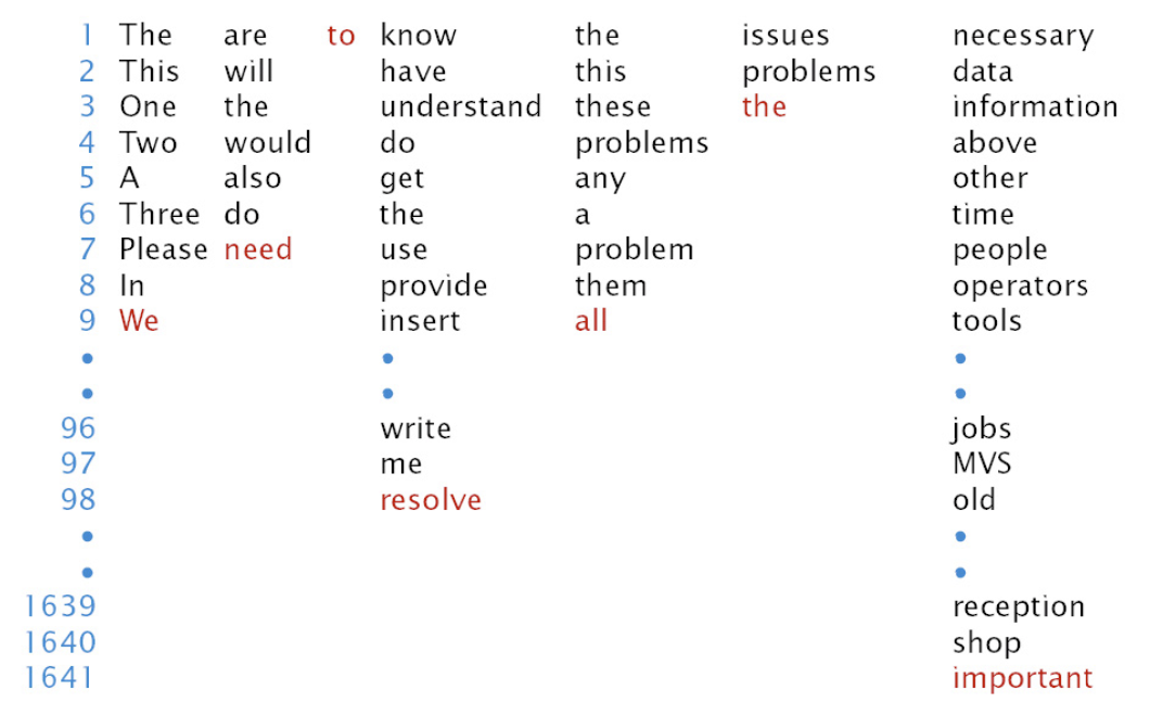
Fig. 148 Trigram Prediction [Jelink 1997]
Evaluation
Qualitatively (How good do random sentences generated from the LM look?)
Evaluate via the task loss/performance measure
Other quantitative intrinsic measure include cross-entropy and perplexity.
Cross-entropy
The (empirical) cross-entropy of a model distribution \(\hat{p}(x)\) with respect to some data \(\boldsymbol{w}=\left\{x_{1}, \ldots, x_{n}\right\}\) is
For an \(n\)-gram LM, to evaluate \(\hat{p}(\cdot)\) on a test set \(\boldsymbol{w}=\left\{w_{1}, \ldots, w_{n}\right\}\).
Perplexity
Recall the perplexity of a distribution \(P(X)\) is \(2^{H_{p}(X)}\).
Here, we consider the empirical perplexity of a model of a distribution w.r.t. a data set
Interpretation: Perplexity is the average number of words possible after a given history (the average branching factor of the LM).
Usually, as \(n\) increases in \(n\)-gram models, perplexity goes down, as we are more certain in the conditional distribution \(p(w_i\vert \phi(\boldsymbol{h_i} ))\)
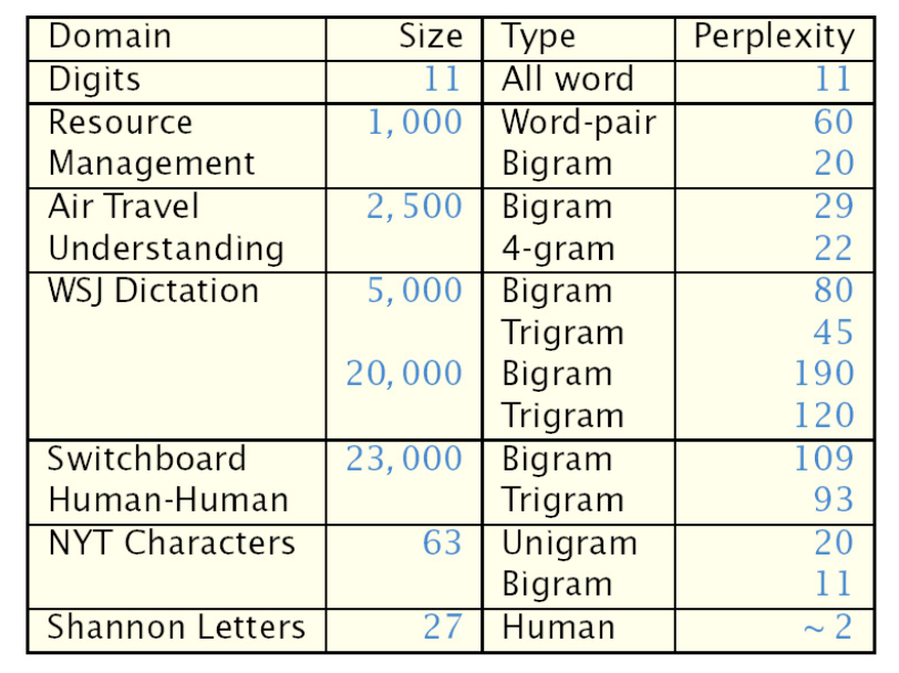
Fig. 149 Perplexity on different domains
Improvement
Sparse Data Problem
A vocabulary of size \(V\) has \(V^n\) possible \(n\)-grams \(w_i \vert w_{i-(n-1)}, \ldots, w_{i-1}\). Most of \(n\)-grams are rare. In a training set, it’s unlikely that we will see all of them. As a result, maximum-likelihood just assign 0 probability.
To alleviate this, we use smoothing: A set of techniques for re-distributing probability mass from frequently seen to unseen/rare events.
Increase probability of unseen/rare \(n\)-grams
therefore, decrease probability of frequently seen \(n\)-grams
Experimental findings: Church and Gale (1992) split a 44 million word data set into two halves. For a bigram that occurs, e.g., 5 times in the first half, how many times does it occur in the second half?
Maximum-likelihood prediction: 5
Actual: ∼ 4.2 < 5
This is because both halves are samples, not identical. There must be some bigrams in 2nd half that are unseen in 1st half, which take up some counts, such that \(5\) is diluted.
There are several improvements to solve this problem.
Laplace (add-one) Smoothing
Simplest idea: Add count of 1 to each event (seen or unseen)
Unigram
Unsmoothed: \(p(w_i) = \frac{C(w_i)}{N}\), where \(N\) is the total number of training word tokens and \(C(\dot)\) is the count.
Smoothed: \(p(w_i) = \frac{C(w_i)+1}{N+V}\), where \(V\) is the vocabulary size
Bigram
Unsmoothed: \(p\left(w_{i} \mid w_{i-1}\right)=\frac{C\left(w_{i-1} w_{i}\right)}{C\left(w_{i-1}\right)}\)
Smoothed: \(p\left(w_{i} \mid w_{i-1}\right)=\frac{C\left(w_{i-1} w_{i}\right)+1}{C\left(w_{i-1}\right)+V}\)
A simple extension is “delta smoothing”: Add some value \(\delta\) instead of \(1\)
Back-off n-grams
Idea: reduce \(n\), so the total number of probabilities to be estimated, which is \(V^n\), decreases.
Use maximum likelihood estimate if we have enough examples; otherwise, back off to a lower-order model:
\[\begin{split} p_{b o}\left(w_{i} \mid w_{i-1}\right) \left\{\begin{array}{ll} p_{\boldsymbol{ML}}\left(w_{i} \mid w_{i-1}\right), & \text { if } C\left(w_{i-1} w_{i}\right) \geq C_{\min } \\ \alpha_{w_{i-1}} p\left(w_{i}\right), & \text { otherwise } \end{array}\right. \end{split}\]where \(\alpha_{w_{i-1}}\) is chosen such that the probability sum to 1
Or, interpolate between higher-order and lower-order \(n\)-gram probabilities
\[ p_{b o}\left(w_{i} \mid w_{i-1}\right) = \lambda p_{\boldsymbol{ML}}\left(w_{i} \mid w_{i-1}\right)+ (1-\lambda) p\left(w_{i}\right) \]
Neural Language Model
Word Embeddings + MLP
To alleviate the sparse data problem in \(n\)-gram model, instead of smoothing, neural language models (multi-layer perceptron) represent each word as a continuous-valued vector (word embedding) given by matrix \(\boldsymbol{C}\), where each row is a word embedding. The embedding is trained.
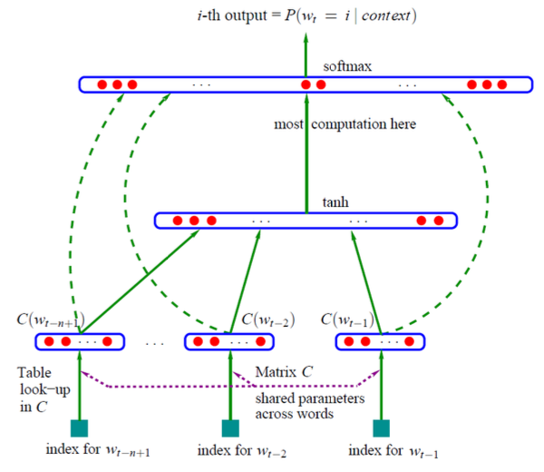
Fig. 150 Neural language models [Bengio 2003]. Dash lines are optional concatenation
The perplexity is reduced from smoothing method’s 312 to 252.
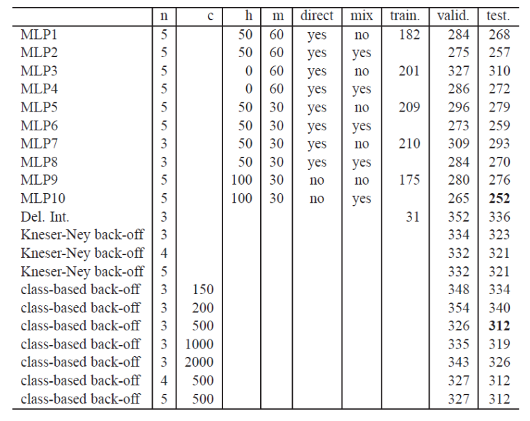
Fig. 151 NLM perplexity
Character Embedding + RNN
Consider a basic RNN language model, that take a character as input, and predict the next character.
Forward propagation:
Objective:
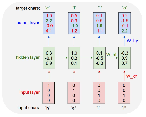
Fig. 152 A basic RNN language model
This is a many-to-many RNN. For details of RNN, see sequential models,
Most recent work based on transformers, trained on much more data, with many more parameters. Example: GPT-3 from OpenAI with 100s of billions of training text tokens + 175 billion parameters