Agglomerative Methods
Unlike \(k\)-means which specify \(k\) at start, agglomerative methods view each data point as a cluster, and then iteratively merge two closest clusters according to some distance measure, until some convergence criterion.
Distance Measure
Euclidean
Let \(A\) and \(B\) be two clusters and let \(a, b\) be individual data points. Usually, \(\operatorname{dist}(a, b)\) is the Euclidean distance, while \(\operatorname{dist}(A, B)\) varies in definitions.
Single-linkage uses the minimum distance
\[\operatorname{dist}(A, B)=\min _{a \in A, b \in B} \operatorname{dist}(a, b)\]Single-linkage tends to yield long, “stringy” clusters.
Complete-linkage uses the maximal distance
\[\operatorname{dist}(A, B)=\max _{a \in A, b \in B} \operatorname{dist}(a, b)\]Complete-linkage tends to yield compact, “round” clusters.
Average-linkage uses the average distance
\[\operatorname{dist}(A, B)=\operatorname{mean} _{a \in A, b \in B} \operatorname{dist}(a, b)\]Wald’s methods uses the increment in total within-group difference if we merge them
\[\begin{split} \begin{aligned} \operatorname{dist}(A, B) &=\sum_{i \in A \cup B}\left\|\boldsymbol{x}_{i}-\boldsymbol{\mu}_{A \cup B}\right\|^{2}-\sum_{i \in A}\left\|\boldsymbol{x}_{i}-\boldsymbol{\mu}_{A}\right\|^{2}-\sum_{i \in B}\left\|\boldsymbol{x}_{i}-\boldsymbol{\mu}_{B}\right\|^2 \\ &=\frac{|A||B|}{|A|+|B|}|| \boldsymbol{\mu}_{A}-\boldsymbol{\mu}_{B}||^{2} \end{aligned} \end{split}\]Wald’s method vs \(k\)-means
At each merge step, Ward’s method minimizes the same sum-of-squares criterion as \(k\)-means, but constrained by choices in previous iterations, so the total sum-of-squares for a given \(k\) is normally larger for Ward’s method than for \(k\)-means.
A common trick: Use Ward’s method to pick \(k\), then run \(k\)-means starting from the Ward cluster
The choice of the measure of dissimilarity matters and has effect on the cluster structure.
Single linkage merges two clusters when one pair of items are close, even though other pairs may be far apart. Thus single linkage clusters could be more spread out.
Complete linkage, on the other hand, could produce more compact cluster.
Average linkage strikes a balance, however sensitive to monotone changes of the similarity measure.
In the examples below, \(k\)-means tends to produce clusters with spherical shapes, and we can see how single-linkage is good or bad.
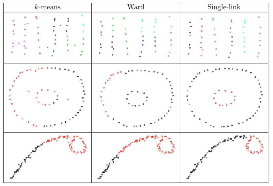
Fig. 119 Comparison of clustering algorithms [Livescue 2021]
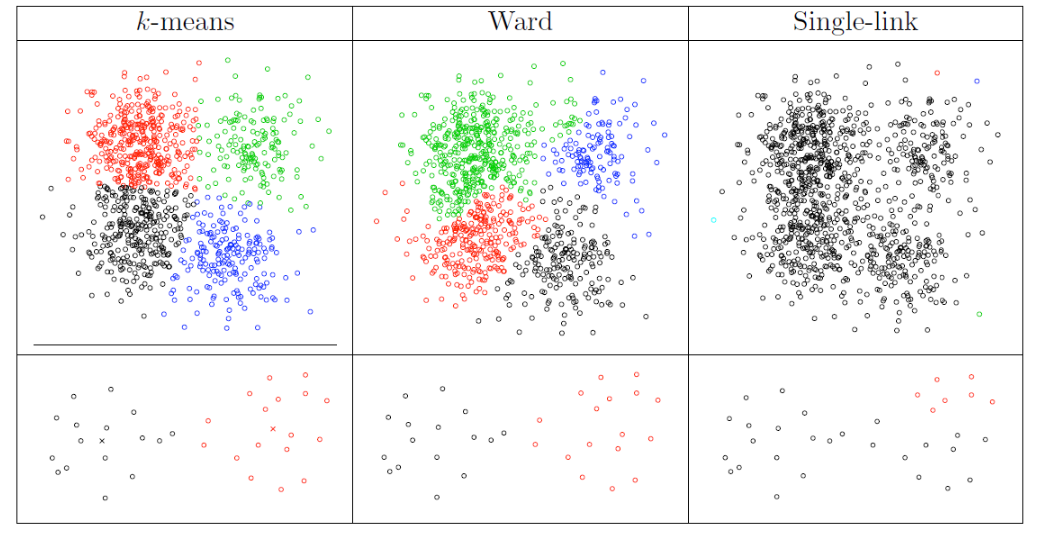
Fig. 120 Comparison of clustering algorithms [Livescue 2021]
Graph-based
For graphs, or induced graphs from data matrix, there are more methods to define \(\operatorname{dist}(a, b)\) for vertices \(a\) and \(b\).
Neighborhood dissimilarity
\[ \operatorname{dist}(a, b) = \frac{\left\vert N(a) \Delta N(b) \right\vert}{d_{(N_v)} + d_{(N_v - 1)}} \]where
\(N(a), N(b)\) are the neighbors of \(a\) and \(b\) respectively.
\(\Delta\) indicates the symmetric difference of two sets. For instance, \(S_1 \Delta S_2 = (S_1 - S_2) \cup (S_2 - S_1)\).
\(d_{(i)}\) is the \(i\)-th smallest element in the degree sequence. The denominator is used to normalize the distance to \([0, 1]\), where 0 and 1 indicate perfect similarity and dissimilarity respectively.
Adjacency matrix euclidean distance
\[ \operatorname{dist}(a, b) = \sqrt{\sum_{k \ne a, b} (A_{ak} - A_{bk})^2} \]which measures the Euclidean distance between rows \(a\) and \(b\) in the adjacency matrix.
Modularity Measure
Besides the distance measures between two sets of vertices, Newman [SAND 294, 297] seeks to greedily optimize the so-called modularity of a partition. Let
\(\mathcal{C} = \left\{ C_1, \ldots, C_K \right\}\) be a given candidate partition.
\(f_{ij}(\mathcal{C}) = \frac{E(C_i, C_j)}{E(G)}\) be the fraction of edges in \(G\) that connect vertices in \(C_i\) with vertices in \(C_j\)
\(\boldsymbol{F}\) be a \(K \times K\) matrix storing the \(f_{ij}\) values, which is symmetric for undirected graphs and can be asymmetric for undirected graphs.
The modularity of \(\mathcal{C}\) is defined as
where \(\mathbb{E}\left( f_{k k} \right)\) is the expected value of \(f_{kk}\) under some random graph model. For instance, if we use a model where a graph is constructed to have the same degree distribution as \(G\), but with edges placed at random, then \(\mathbb{E}\left( f_{k k} \right) = f_{k+} \cdot f_{+k}\) where \(f_{k+}\) and \(f_{+k}\) are the \(k\)-th row and column sums of \(\boldsymbol{F}\).
Large values of \(\bmod (\mathcal{C})\) suggest that \(\mathcal{C}\) captures nontrivial structure.
Optimization of the modularity function is NP-complete problem. A greedy agglomerative algorithm is therefore commonly used for heuristic optimization, which runs in \(\mathcal{O} (N_v ^2 \log N_v)\) time generally, using sophisticated data structures, but nearly linear time on sparse networks with hierarchical structure, making it appealing for use in the context of certain large networks.
Convergence Criterion
A good representation of clustering process is dendrogram. The \(x\)-axis represents items, and the distance along \(y\)-axis between two connected items is proportional to the dissimilarity between two clusters at the two connected items. It provides visual guidance to a good choice for the number of clusters
Stop merging when
the merge cost (distance between merged clusters) would be much larger than in previous iterations (for some precise definition of “much larger”), or
the modularity \(\bmod (\mathcal{C})\) is maximized optimal partition.
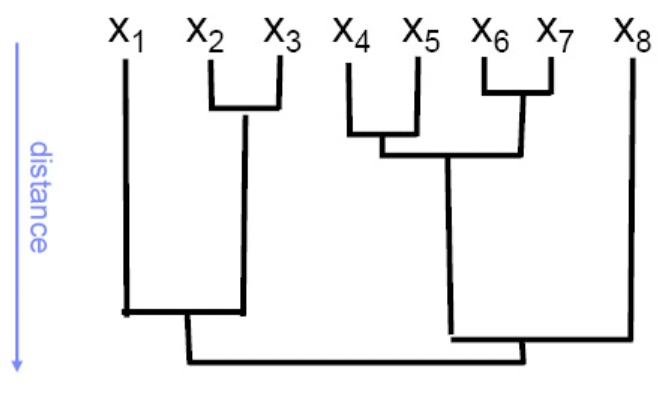
Fig. 121 Representing clustering with dendrograms
Examples
Given an \(n \times p\) matrix of \(p\) variables and \(n\) features, we can do two clusterings
clustering of the \(p\) variables, where distance is \(d = \sqrt{2 (1-\rho)}\)
clustering of the \(n\) observations, where distance can be Euclidean distance (of normalized variable values), etc.
For instance, given a matrix of phonemes and electrodes, we are interested in discovering cohesive neural regions/firing patterns and relating them to clusters of stimuli.
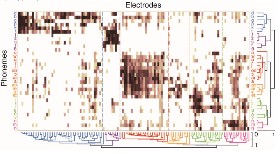
Fig. 122 Cohesive neural regions/firing patterns [Bouchard et al. 2013]