Multidimensional Scaling¶

In this section we introduce (metric) multidimensional scaling (MDS). It finds some representation of input data, which can be used for dimension reduction or visualization. In addition to a $n \times d$ data matrix $\boldsymbol{X}$, MDS can also take pairwise relations, aka proximity data, as input, such as

pairwise dissimilarity measures of data points as input, denoted $\boldsymbol{D} \in \mathbb{R} ^{n \times n}$
- a matrix of Euclidean distances between data points
- a matrix of city-city airline distance (not necessarily Euclidean)
- survey results of customers’ perception of dissimilarity between products
Note that the input dissimilarity matrix $\boldsymbol{D}$ may not be exactly euclidean distance, hence it does not enjoy all properties that a distance matrix has.
pairwise similarity measures of data points as input, denoted $\boldsymbol{S} \in \mathbb{R} ^{n \times n}$
- co-occurrence counts of words between documents
- an adjacency matrix of web pages (MDS as a graph layout technique)
- survey results of customers’ perception of similarity between products
Usually the diagonal entires of a dissimilarity matrix are $0$, and those of a similarity matrix are 1. A dissimilarity measure can be created based on the given similarity measure, and vice versa.

On similarity, dissimilarity, proximity, distance

Similarity measure reflects how close two objects are. The closer the two objects are to each other, the larger is their similarity value.
Dissimilarity measure indicates how different two objects are. The farther the two objects are to each other, the larger is their dissimilarity value.
Proximity can be either similarity or dissimilarity.
Distance sometime loosely refers to a dissimilarity measure. On the other hand, distance as a metric is a more strictly defined mathematical concept.

In total, there are four types of MDS: {metric, non-metric} $\times$ {distance, classical}.

distance scaling: fit dissimilarity by Euclidean distance $d_{ij} \approx \left\| \boldsymbol{z} _i - \boldsymbol{z} _j \right\|$
classical scaling: transform dissimilarity to some form of ‘similarity’ and then fit by inner product $s_{ij} \approx \langle \boldsymbol{z}_i , \boldsymbol{z} _j \rangle$. Note the identity $\left\| \boldsymbol{z}_i - \boldsymbol{z}_j \right\| ^2 = \left\| \boldsymbol{z} _i \right\|^2 + \left\| z _j \right\| ^2 - 2 \langle \boldsymbol{z}_i , \boldsymbol{z}_j \rangle$.
metric scaling uses actual numerical values of dissimilarities
non-metric scaling applies ranks, KL divergences, etc. rather than numerical dissimilarities.

Here, we introduce metric classical scaling. For others, see this paper.

Many non-linear dimensionality reduction methods are extension to MDS. MDS is a clue to link linear and non-linear dimensionality reduction.

Objective¶

Given a distance matrix $\boldsymbol{D}\in \mathbb{R} ^{n \times n}$, can we find a $2$-dimensional representation of it $\boldsymbol{Z} \in \mathbb{R} ^{n \times k}$, to visualize them in 2-D plane?

More generally, suppose $\boldsymbol{Z} \in \mathbb{R} ^{n \times k}$ are the underlying embeddings, MDS finds $\boldsymbol{Z}$ such that the distance is nearly preserved: $\left\| \boldsymbol{z} _i - \boldsymbol{z} _j \right\| \approx d_{ij}$. Hence the objective is to find embeddings $\boldsymbol{Z}$ that minimizes stress

\[ \operatorname{Stress}_{D}\left(\boldsymbol{z}_{1}, \ldots, \boldsymbol{z}_{N}\right)=\left(\sum_{i \neq j=1}^n\left(d_{ij}-\left\|\boldsymbol{z}_{i}-\boldsymbol{z}_{j}\right\|\right)^{2}\right)^{1 / 2} \]
Given a distance matrix $\boldsymbol{D}$, find coordinates for the $n$ points in a low dimensional space such that the corresponding distances maintain the ordering of pairwise distance in $\boldsymbol{D}$.

Given data matrix $\boldsymbol{X} \in \mathbb{R} ^{n \times d}$ with zero column means, as a dimensionality reduction method, MDS seeks a $k$-dimensional representation $\boldsymbol{Z} \in \mathbb{R} ^{n \times k}$ that preserves inner products (a similarity measure) between pairs of data points $(\boldsymbol{x_i}, \boldsymbol{x}_j)$

\[ \min \sum_{i, j}\left(\boldsymbol{x}_{i} ^\top \boldsymbol{x}_{j}-\boldsymbol{z}_{i} ^\top \boldsymbol{z}_{j}\right)^{2} \]

or equivalently

\[ \min \left\Vert \boldsymbol{X} \boldsymbol{X} ^\top - \boldsymbol{Z} \boldsymbol{Z} ^\top \right\Vert _F^2 \]

The lower-dimensional embeddings can be then used for downstream tasks, including clustering, classification, etc. It worths mentioning that the embeddings are exactly the same as PCA’s. See the last section for proof.

Learning¶

Depending on how we formulate the objective, there are mainly two methods.

Spectral Decomposition¶

Let $\boldsymbol{C} = \boldsymbol{I}-\frac{1}{n} \boldsymbol{1} \boldsymbol{1}^{\top}$ be a centering matrix.

If the input matrix is data matrix $\boldsymbol{X}$, the solution can be obtained from the $n\times n$ Gram matrix $\boldsymbol{G}$ of inner products of centered data $\bar{\boldsymbol{X} }= \boldsymbol{C} \boldsymbol{X}$ with zero column means, where $\boldsymbol{C} = (\boldsymbol{I} - \frac{1}{n} \boldsymbol{1} \boldsymbol{1} ^{\top})$.

\[ \boldsymbol{G} := \bar{\boldsymbol{X}} \bar{\boldsymbol{X}} ^\top \]

where $g_{i j}=\bar{\boldsymbol{x}}_{i} \bar{\boldsymbol{x}}_{j} ^{\top}$. Recall our objective is preserve inner product

\[ \min \left\Vert \bar{\boldsymbol{X}} \bar{\boldsymbol{X}} ^\top - \boldsymbol{Z} \boldsymbol{Z} ^\top \right\Vert _F^2 \]

Hence it is natural to approximate $\boldsymbol{G}$ by spectral method. Suppose the spectral decomposition of $\boldsymbol{G}$ is $\boldsymbol{G} = \boldsymbol{V} \boldsymbol{\Lambda} \boldsymbol{V} ^\top$, then the $k$-dimensional representation is given by

\[ \boldsymbol{Z}_{n \times k} = \left[ \boldsymbol{V} \boldsymbol{\Lambda} ^{1/2} \right]_{[:k]} = \boldsymbol{V}_{[: k]} \boldsymbol{\Lambda}_{[: k,: k]}^{1 / 2} \]

For derivation see here. The reconstruction of $\boldsymbol{G}$ from $\boldsymbol{Z}$ is then $\widehat{\boldsymbol{G}} = \boldsymbol{Z} \boldsymbol{Z} ^\top$.
If the input is a similarity matrix $\boldsymbol{S}$, we can run the above algorithm by treating $\boldsymbol{S}$ as $\boldsymbol{G}$. Some other methods first convert a similarity measure to a distance measure and then analyze it. There are many ways for such conversion, e.g. $d = 10 \sqrt{2 (1-s)}$, which guarantees that the obtained dissimilarity order is exactly the inversion of the similarly order.
If the input is an Euclidean distance matrix $\boldsymbol{D}$, suppose the true data is $\boldsymbol{X}$, then by definition we have

\[ d_{i j}=\left\|\boldsymbol{x}_{i}-\boldsymbol{x}_{j}\right\|^{2}=\left\|\boldsymbol{x}_{i}\right\|^{2}-2 \boldsymbol{x}_{i}^{\top} \boldsymbol{x}_{j}+\left\|\boldsymbol{x}_{j}\right\|^{2} \]

We can convert the Euclidean distance matrix $\boldsymbol{D}$ to the Gram matrix $\boldsymbol{G}$ for centered $\boldsymbol{X}$ by left- and right-multiplying $\boldsymbol{C}$

\[ \boldsymbol{G} = - \frac{1}{2} \boldsymbol{C} (\boldsymbol{D} * \boldsymbol{D} )\boldsymbol{C} ^{\top} \]

where $[\boldsymbol{D} * \boldsymbol{D}]_{ij} = d_{ij}^2$. Then we can run MDS over $\boldsymbol{G}$ to obtain $k$-dimensional representation. Note that since $\boldsymbol{G}$ is row-centered, it has an eigenvalue 0. Hence, the maximal possible value of $k$ is $d-1$, rather than $d$.

Proof

\[\begin{split}\begin{aligned} d_{ij}^2 &= \left\| x_i \right\|^2 + \left\| x_j \right\|^2 - 2 \boldsymbol{x}_i ^{\top} \boldsymbol{x}_j \\ \Rightarrow \boldsymbol{D} * \boldsymbol{D} &= \boldsymbol{v} \boldsymbol{1} ^{\top} + \boldsymbol{1} \boldsymbol{v} ^{\top} - 2 \boldsymbol{X} \boldsymbol{X} ^{\top}\text{ where } v_i = \left\| \boldsymbol{x}_i \right\| ^2 \\ \Rightarrow \boldsymbol{C} (\boldsymbol{D} * \boldsymbol{D}) \boldsymbol{C} &= -2 \boldsymbol{C} \boldsymbol{X} \boldsymbol{X} ^{\top} \boldsymbol{C} \quad \because \boldsymbol{C} (\boldsymbol{v} \boldsymbol{1} ^{\top}) \boldsymbol{C} = 0\\ \Rightarrow -\frac{1}{2} \boldsymbol{C} (\boldsymbol{D} * \boldsymbol{D}) \boldsymbol{C} &= \bar{\boldsymbol{X}} \bar{\boldsymbol{X}} ^{\top} \\ &= \boldsymbol{G} \end{aligned}\end{split}\]

$\square$
Motivated by this, if the input matrix is dissimilarity (not necessarily Euclidean distance) matrix $\boldsymbol{D}$, we can run the above algorithm over $\boldsymbol{B} = - \frac{1}{2} \boldsymbol{C} \boldsymbol{D} \boldsymbol{C}$, where $\boldsymbol{B}$ approximates $\boldsymbol{G}$.

Hence can see, this spectral method is particularly appropriate when the dissimilarities are actually or at least approximately Euclidean distances.

Warning

Since the dissimilarity measure may not be Euclidean, $\boldsymbol{B}$ may have some negative eigenvalues. The maximal possible value of $k$ is then the number of of positive eigenvalues of $\boldsymbol{B}$.

This spectral method also uses principal components (eigenvectors) like PCA. Therefore sometimes classical MDS is also called “principal coordinates analysis”.

Gradient Descent¶

If we have some non-trivial objective function, say some measure of the goodness-of-fit of the lower dimensional representation $\boldsymbol{Z} \in \mathbb{R}^{n \times k}$, then the measure can be viewed as a loss function on $\mathbb{R} ^{n \times k}$. The optimization algorithm can be carried out by numerical methods such as gradient descent.

Practical Issues¶

Goodness of Fit¶

We can use (scaled) stress [Kruskal 1964] to measure the goodness-of-fit of the lower dimensional representation, whose value is in range [0, 1].

\[ \operatorname{Stress}_ \boldsymbol{D} (k) = \left\{ \frac{\sum_{i \ne j} (d_{ij} - \hat{d}_{ij})^2}{\sum_{i \ne j} d_{ij}^2} \right\} ^{-1/2} \]

$d_{ij}$ are the entries in distance matrix $\boldsymbol{D}$, presumably the distance of the two objects in a higher dimensional space
$\hat{d}_{ij} = \left\| \boldsymbol{z} _i - \boldsymbol{z} _j \right\|_2$ is the Euclidean distance in the $k$-dimensional space (or some other distance measure).

An alternative measure SStress developed by Takane 1997 is

\[ \operatorname{SStress}_{\boldsymbol{D} }(k) = \left\{ \frac{\sum_{i \ne j} (d_{ij}^2 - \hat{d}_{ij}^2)^2}{\sum_{i \ne j} d_{ij}^4} \right\} ^{1/2} \]

Typically the value of Stress or SStress less than 0.1 is considered a good representation of the objects by the points in the given low dimension configuration. In practice, the goodness of fit of Stress is based on the range of the values:

\[\begin{split} \begin{array}{c||c|c|c|c|c} & \text { Perfect } & \text { Excellent } & \text { Good } & \text { Fair } & \text { Poor } \\ \hline \text { Stress value } & 0 \% & 2.5 \% & 5 \% & 10 \% & 20 \% \end{array} \end{split}\]

Besides a scalar measure, we can also plot the fitted distance $\hat{d}_ij$ over the input distance $d_{ij}$. If the points on the $45^\circ$ $y=x$ line, then the distances are preserved. See the plots in next section.

Tuning¶

How to choose optimal $k$? We can see how the goodness-of-fit mentioned above varies with $k$.

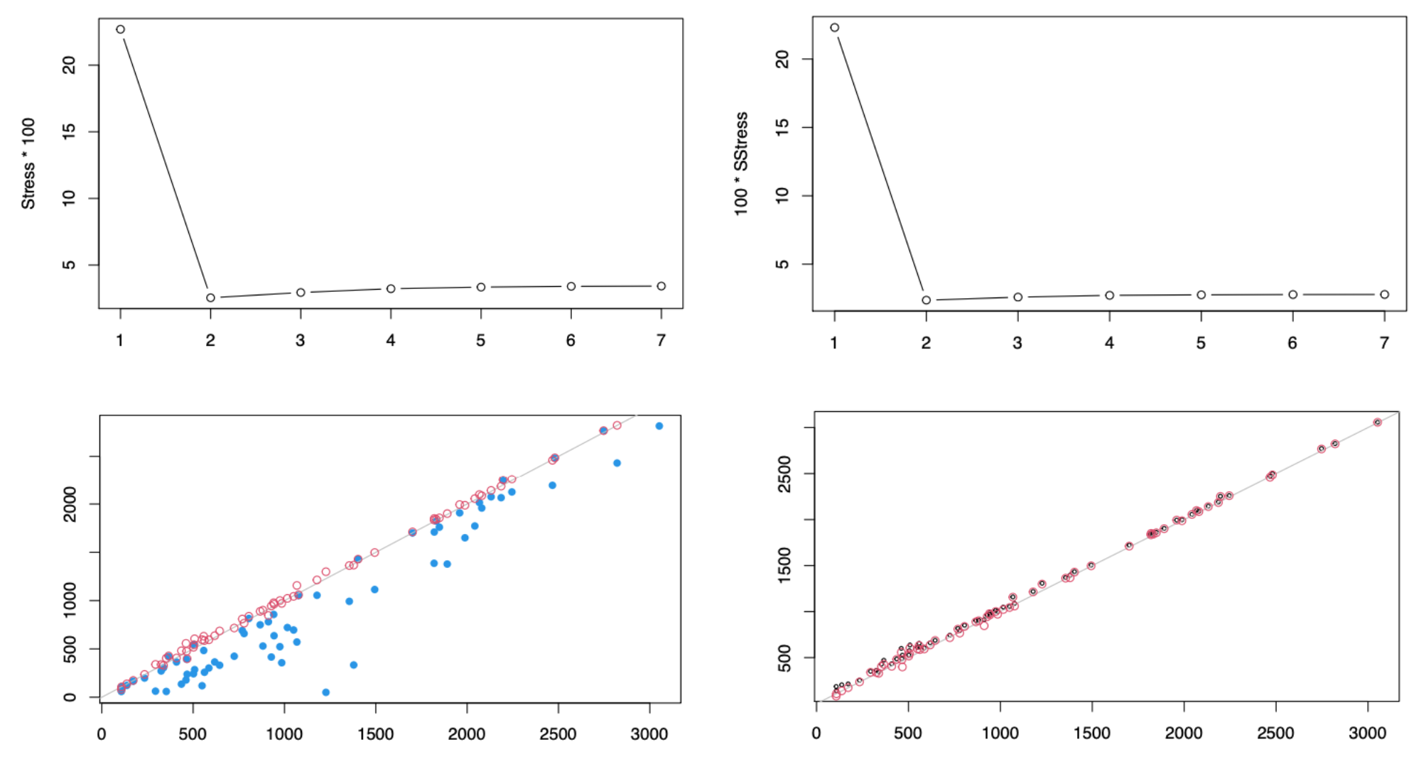
Fig. 102 Stress plots (upper row) and fitted vs real distance plots (lower row). .¶

Both Stress and SStress drop when $k=1$ changes to $k=2$, but both increase afterwards, i.e. the loss is not monotonically decreasing as $k$ becomes large!
We plot fitted distance for $k=1$ (blue), $k=2$ (red), $k=8$ (black). When $k=1$, the fitting is poor. When $k=2$, the fitting is already quite good. As $k$ increases, the points roughly stay unchanged, i.e. no obvious improvement. The results are consistent with the stress results.

Note that the maximal possible $k$ is also related to the rank of the input distance matrix $\boldsymbol{D}$.

Relation to PCA¶

We compare PCA and MDS in terms of finding representation $\boldsymbol{Z}$ given $\boldsymbol{X}$,

Difference: unlike PCA which gives a projection equation $\boldsymbol{z} = \boldsymbol{U} ^\top \boldsymbol{x}$, MDS only gives a projected result for the training set. It does not give us a way to project a new data point.
Connections
- the two representation are exactly the same. Suppose the data matrix $\boldsymbol{X}$ is centered. Let $\boldsymbol{Z} _{PCA}$ be the $n\times k$ projected matrix by PCA and $\boldsymbol{Z} _{MDS}$ be that by MDS. Then it can be shown that
  
  \[\begin{split} \boldsymbol{Z} _{PCA} = \boldsymbol{Z} _{MDS}\\ \end{split}\]
  
  This also implies that, to obtain PCA projections, we can use the covariance matrix, the Gram matrix $\boldsymbol{G}$, or the Euclidean distances matrix $\boldsymbol{F}$.
  Proof
  
  Consider the SVD of the centered data matrix
  
  \[\boldsymbol{X}_{n\times d} = \boldsymbol{V} \boldsymbol{\Sigma} \boldsymbol{U} ^\top\]
  - In PCA, the $n\times d$ embedding matrix is
    
    \[ \boldsymbol{Z}_{PCA} = \boldsymbol{X} \boldsymbol{U} \]
  - In MDS, the EVD of the inner product matrix $\boldsymbol{G}$ is
    
    \[ \boldsymbol{G}_{n \times n} = \boldsymbol{X} \boldsymbol{X} ^\top = \boldsymbol{V} \boldsymbol{\Sigma} \boldsymbol{\Sigma} ^\top \boldsymbol{V} ^\top = \boldsymbol{V} \boldsymbol{\Lambda} \boldsymbol{V} ^\top = \boldsymbol{V} _{[:d]} \boldsymbol{D} \boldsymbol{V} _{[:d]} ^\top \]
    
    where
    
    \[\begin{split} \boldsymbol{\Lambda} _{n \times n} = \left[\begin{array}{cc} \boldsymbol{D} _{d \times d} & \boldsymbol{0} \\ \boldsymbol{0} & \boldsymbol{0}_{(n-d) \times (n-d)} \end{array}\right] \end{split}\]
    
    The embedding matrix is
    
    \[ \boldsymbol{Z} _{MDS} = \boldsymbol{V}_{[:d]} \boldsymbol{\Lambda} ^{1/2}_{[:d, :d]} = \boldsymbol{V}_{[:d]} \boldsymbol{D} ^{1/2} \]
  Substituting the SVD of $\boldsymbol{X}$ to the $\boldsymbol{Z} _{PCA}$ gives
  
  \[\begin{split}\begin{aligned} \boldsymbol{Z} _{PCA} &= \boldsymbol{X} \boldsymbol{U}\\ &= \boldsymbol{V} \boldsymbol{\Sigma} \boldsymbol{U} ^{\top} \boldsymbol{U} \\ &= \boldsymbol{V} \boldsymbol{\Sigma}_{n \times d}\\ &= \boldsymbol{V}_{[:d]} \boldsymbol{\Sigma}_{[:d, :d]}\\ &= \boldsymbol{V}_{[:d]} \boldsymbol{D}^ {1/2} \quad \because \text{singular value } \sigma_j \ge 0$\\ &= \boldsymbol{Z} _{MDS} \\ \end{aligned}\end{split}\]
- PCA finds basis $\boldsymbol{u} \in \mathbb{R} ^n$ (principle directions) for spanning $\boldsymbol{X}$, and MDS finds the coordinates $\boldsymbol{z} \in \mathbb{R} ^d$ of the embeddings associated with the PCA basis.
  
  \[\begin{split}\begin{aligned} \boldsymbol{X} ^{\top} &= \boldsymbol{U} (\boldsymbol{V} \boldsymbol{\Sigma} ) ^{\top} \\ &= \boldsymbol{U} (\boldsymbol{V}_{[:d]} \boldsymbol{\Sigma}_{[:d]} ) ^{\top} \\ &= \boldsymbol{U} \boldsymbol{Z} _{MDS} ^{\top} \\ [\boldsymbol{x} _i \ \ldots \ \boldsymbol{x} _n]&= [\boldsymbol{u}_1 \ \ldots \ \boldsymbol{u} _d ] [\boldsymbol{z} _1 \ \ldots \ \boldsymbol{z} _n] \\ \boldsymbol{x} _i&= \sum_{j=1}^d z^{MDS}_{ij} \boldsymbol{u} _j\\ \end{aligned}\end{split}\]

Reference: Davis-kahan theorem

Data Science Handbook