Topology Inference
Can we do inference on graphs (e.g. connectivity) like we can do for usual data matrix? Do we have the concepts and tools such as statistical consistency, efficiency, and robustness? Unfortunately, there is at present no single coherent body of formal results on inference problems over graphs.
The frameworks developed in these settings naturally take various forms, as dictated by context, with differences driven primarily by the nature of the topology to be inferred and the type of data available.
Link Prediction
Given
full knowledge of all the vertices attributes \(\boldsymbol{x}=\left(x_{1}, \ldots, x_{N_{v}}\right)^{\top}\)
status of some of the edges/non-edges \(\boldsymbol{Y}^{obs}\)
Infer
the rest of the edges/non-edges \(\boldsymbol{Y}^{miss}\), using \(\boldsymbol{Y}^{obs}\) and \(\boldsymbol{x}\).
Sometimes we need additional modeling for the mechanisms of missingness.
missing at random: probability of missing \(Y_{ij}\) only depends on the values of those other edge variables
informative missingness: probability of missing \(Y_{ij}\) depends on themselves
A basic framework:
But there are many challenges to predict \(Y_{ij}^{miss}\) jointly. Many methods predict individual \(Y_{ij}^{miss}\), as introduced below.
Scoring
Scoring methods are based on the use of score functions. These methods are less formal than the model-based methods, but can be quite effective, and often serve as a useful starting point.
For each potential edge \((i, j) \in V^{(2)}_{miss}\) , a score \(s(i, j)\) is computed. A set of predicted edges may then be returned by
applying a threshold \(s^*\) to these scores, or
ordering them and keeping those pairs with the top \(n^*\) values
There are many scores, designed to assess certain structural characteristics of a graph \(G^{obs}\).
negative shortest distance \(- \operatorname{dist}_{G^{obs}}(i, j)\): inspired by the small-world principal, the closer the two nodes are, more likely to form an edge
#(common neighbors) \(\left\vert N_i^{obs} \cap N_j^{obs} \right\vert\): more common neighbors, more likely to form an edge
Jaccard coefficient \(\frac{\left\vert N_i^{obs} \cap N_j^{obs} \right\vert}{\left\vert N_i^{obs} \cup N_j^{obs} \right\vert}\): a standardized version of the above value.
Adamic-Adar index \(\sum_{k \in N_{i}^{obs} \cap N_{j}^{o b s}} \log \frac{1}{\left|N_{k}^{o b s}\right|}\): variation of the above, weighting more heavily those common neighbors of \(i\) and \(j\) that are themselves not highly connected with other vertices.
There score functions only assess local structure in \(G^{obs}\). If two nodes do not have any common neighbors, then the score is 0, but they may potentially be connected in \(G^{miss}\).
To fix this, we an use global neighborhood overlap scores
Katz index \(S(i,j) = \sum_{\ell=1}^\infty \beta^\ell [\boldsymbol{A} ^\ell]_{ij}\): count the number of paths of all lengths between a given pair of nodes, and then discounted by factor \(\beta \in (0, 1)\) and sum up. To compute the number of paths, use powers of the graph adjacency matrix \(\boldsymbol{A}\). In fact, it Katz index matrix can be computed in closed-form by geometric series of matrices
\[ \boldsymbol{S} = \sum_{\ell=1}^\infty \beta^\ell \boldsymbol{A} ^\ell = \sum_{\ell=0}^\infty \beta^\ell \boldsymbol{A} ^\ell - \boldsymbol{I} = (\boldsymbol{I} - \beta \boldsymbol{A} ) ^{-1} - \boldsymbol{I} \]
For others defined through spectral characteristics of \(G^{obs}\), see [SAND 261]. Examples:
Classification
Can we approach link prediction as a classification problem?
(binary) labels: \(\boldsymbol{y} ^{obs}\)
features: \(\boldsymbol{x}^{obs}\) and \(\boldsymbol{y} ^{obs}\)
predict: \(\boldsymbol{Y} ^{miss}\).
Logistic Regression
A common choice is logistic regression.
\(\boldsymbol{Z} _{ij}\) is a vector of explanatory variables indexed in the unordered pairs \((i, j)\). In general it is some transformation of \(\boldsymbol{Y} ^{obs}_{(-ij)}\) and/or \(\boldsymbol{X}\):
\[\boldsymbol{Z}_{i j}=\left(g_{1}\left(\boldsymbol{Y}_{(-i j)}^{o b s}, \boldsymbol{X}\right), \ldots, g_{K}\left(\boldsymbol{Y}_{(-i j)}^{o b s}, \boldsymbol{X}\right)\right)^{\top}\]For instance, \(g\) can be
network structure measures using \(\boldsymbol{Y} ^{obs}_{-ij}\), e.g. score functions introduced above
similarity measures between the \(k\)-th vertex attributes of vertex \(i\) and \(j\),
additive \(X_{ik} + X_{jk}\) for continuous values
indicator \(\mathbb{I} \left\{ X_{ik} = X_{jk} \right\}\) for discrete values
the coefficient \(\boldsymbol{\beta}\) is assumed common to all pairs.
- Prediction
We compare the predicted value vs some threshold, e.g. 0.5, and then decide classification.
\[ \mathbb{P}_{\hat{\beta}}\left(Y_{i j}^{miss}=1 \mid \boldsymbol{Z}_{i j}=\boldsymbol{z}\right)= \frac{\exp (\hat{\boldsymbol{\beta} } ^{\top} \boldsymbol{z} )}{1 + \exp (\hat{\boldsymbol{\beta} } ^{\top} \boldsymbol{z} )} \]
Issues
Need to consider the missing mechanism. If \(\boldsymbol{Y} ^{miss}\) is not at random, the accuracy of the classification approach will suffer.
In a graph, \(Y_{ij}\) are usually not independent given explanatory variables \(\boldsymbol{Z}\), which is assumed in logistic models (no formal work to date exploring the implications on prediction accuracy of ignoring possible dependencies in this manner). Introducing latent variable solve this issue, as discussed below
Latent Variables
The use of latent variables is an intuitively appealing way to indirectly model unobserved factors driving the formation of network structure. Let \(\boldsymbol{M}\) be an unknown, random, symmetric \(N_v \times N_v\) matrix of latent variables, defined as
\(\boldsymbol{U}\) is an \(N_v \times N_v\) random orthonormal matrix,
\(\boldsymbol{\Lambda}\) is an \(N_v \times N_v\) random diagonal matrix,
\(\boldsymbol{E}\) is a symmetric matrix of i.i.d. noise variables
Then each entry of \(\boldsymbol{M}\) is
- Intuition
The latent variable matrix \(\boldsymbol{M}\) is intended to capture effects of network structural characteristics or processes not already described by the observed explanatory variables \(\boldsymbol{Z} _{ij}\). We add \(M_{ij}\) as an explanatory variable (like that in random effect models). The model becomes
\[ \log \left[ \frac{\mathbb{P}_{\beta}\left(Y_{i j}=1 \mid \boldsymbol{Z}_{i j}=\boldsymbol{z}, M_{ij}=m\right)}{\mathbb{P}_{\beta}\left(Y_{i j}=0 \mid \boldsymbol{Z}_{i j}=\boldsymbol{z}, M_{ij}=m\right)} \right]=\beta^{\top} \boldsymbol{z} + m \]Now \(Y_{ij}\) are conditionally independent given \(\boldsymbol{Z} _{ij}\) and \(\boldsymbol{M} _{ij}\), but conditionally dependent given only the \(\boldsymbol{Z} _{ij}\).
Commonly used distributions for \(\boldsymbol{U} , \boldsymbol{\Lambda} , \boldsymbol{E}\).
\(\boldsymbol{U}\): uniform distribution on the space of all \(N_v \times N_v\) orthonormal matrices
\(\boldsymbol{\Lambda} , \boldsymbol{E}\): multivariate Gaussian (facilitate MCMC sampling)
- Prediction
Compare the expected probability of \(Y_{ij}=1\) with some threshold, which may be approximated numerically to any desired accuracy by the corresponding sample average of draws from the posterior indicated
\[ \mathbb{E}\left(\frac{\exp \left\{\beta^{T} \boldsymbol{Z}_{i j}+M_{i j}\right\} }{1+\exp \left\{\beta^{T} \boldsymbol{Z}_{i j}+M_{i j}\right\}} \mid \boldsymbol{Y}^{o b s}=\boldsymbol{y}^{o b s}, \boldsymbol{Z}_{i j}=\boldsymbol{z}\right) \]- Cons
MCMC computation cost, mainly driven by the need to draw \(N_v ^2\) unobserved variables \(U_{ij}\). Sol: let \(\boldsymbol{U}\) have only \(K\) non-zero column vectors for \(K \ll N_v\), hence low-rank of \(\boldsymbol{M}\). In fact \(K=2, 3\) work well in practice. [SAND 200, 201]
For a case study see [SAND pg.205].
Association Networks
We use non-trivial level of association (e.g. correlation) between certain characteristics of the vertices to decide edge assignment. But the association is itself unobserved and must be inferred from measurements reflecting these characteristics.
Given
no knowledge of edge status anywhere
relevant measurements at all of the vertices \(\left\{ \boldsymbol{x}_1, \ldots, \boldsymbol{x}_{N_v} \right\}\)
Infer
edge status \(\boldsymbol{Y}\) using these measurements \(\boldsymbol{x}\)
Correlation Networks
An intuitive measure of similarity between a vertex pair \((i, j)\) is correlation.
Buildup
Suppose for each vertex \(i\), we have \(n\) independent observations \(\left\{ x_{i1}, \ldots, x_{in} \right\}\), e.g. gene expression levels from \(n\) experiments. We can then form an \(n \times N_v\) matrix \(\boldsymbol{X}\), and compute the \(N_v \times N_v\) sample covariance matrix \(\boldsymbol{S}\), hence obtain the entries \(\hat{\sigma}\) and use that to compute \(\hat{\rho}\).
The corresponding association graph \(G\) is the graph with edge set
Hence, the the task is to infer the set of non-zero correlations, which can be approached through hypotheses testing
Problems
what test statistics?
what is the null distribution of that test statistic?
there are \(N_v (N_v - 1)/2\) potential edges, which implies multiple testing problem.
Testing
If \((X_i, X_j)\) follow bivariate Gaussian, then \(\hat{\rho}_{ij}\) under \(H_0: \rho_{ij}=0\) has a closed-form, but the computation of \(p\)-values is hard. Therefore, some transformed versions of \(\hat{\rho}_{ij}\) may be preferable
\(z_{i j}=\frac{\hat{\rho}_{i j} \sqrt{n-2}}{\sqrt{1-\hat{\rho}_{i j}^{2}}} \sim t_{n-1}\), and under \(H_0\) it is robust to departures of \(X_i\) from Gaussianity.
\(z_{i j}=\tanh ^{-1}\left(\hat{\rho}_{i j}\right)=\frac{1}{2} \log \left[\frac{\left(1+\hat{\rho}_{i j}\right)}{\left(1-\hat{\rho}_{i j}\right)} \right]\), aka Fisher transformation.
for bivariate Gaussian pairs, the distribution of \(z_{ij}\) does not have a simple exact form. But under \(H_0\) this distribution is well approximated by \(\mathcal{N} (0, \frac{1}{n-3} )\) even for moderately large \(n\).
Permutation methods can also be used, but is computationally intensive for large \(N_v\).
Multiple Testing
Recall the false discovery rate is defined to be
where \(R\) is the number of rejections among our tests and \(R_{\text {false }}\) is the number of false rejections.
To guarantee \(\mathrm{FDR} \le \gamma\), we use the original method proposed by Benjamini and Hochberg [SAND 33],
sort the \(p\)-values from our \(N =N_v (N_v−1)/2\) tests, yielding a sequence \(p_{(1)}\le p_{(2)} \le \ldots \le p_{(N)}\),
reject the null hypothesis for all potential edges for which \(p_{(k)} \leq(k / N) \gamma\).
Alternatively, we can use Storey [SAND 370] method and declare edges to be present using a particular \(q\)-value. Then only \(qN\) of the edges will be included erroneously.
When dependency of tests [??] exists, the first method still holds, and there are other methods.
Partial Correlation Networks
If it is felt desirable to construct a graph \(G\) where the inferred edges are more reflective of direct influence among vertices, rather than indirect influence through some common neighbor (confounders), the notion of partial correlation becomes relevant.
Partial Correlation
Continuing from the setting of \(n \times N_v\) measurement matrix \(\boldsymbol{X}\).
- Definition (Partial correlation)
The partial correlation of attributes \(X_i\) and \(X_j\) of vertices \(i, j \in V\) w.r.t. the attributes \(X_{k_1}, \ldots, X_{k_m}\) of vertices \(k_1, \ldots, k_m \in V \setminus \left\{ i, j \right\}\), is the correlation between \(X_i\) and \(X_j\) left over, after adjusting for those effects common to both. Let \(S_m = \left\{ k_1, \ldots, k_m \right\}\), the partial correlation of \(X_i\) and \(X_j\) adjusting for \(\boldsymbol{X} _{S_m} = [X_{k_1}, \ldots, X_{k_m}] ^{\top}\) is defined as
\[ \rho_{i j \mid S_{m}}=\frac{\sigma_{i j \mid S_{m}}}{\sqrt{\sigma_{i i\mid S_{m}} \sigma_{j j \mid S_{m}}} } \]
To compute it, let \(\boldsymbol{W} _1 = [X_i, X_j] ^{\top}\) and \(\boldsymbol{W} _2 = \boldsymbol{X} _{S_m}\). We can partition the covariance matrix to
Then the \(2 \times 2\) partial covariance matrix is
The values \(\sigma_{ii\vert S_m}, \sigma_{jj\vert S_m}\) and \(\sigma_{ij\vert S_m} = \sigma_{ji\vert S_m}\) are diagonal and off-diagonal elements of \(\boldsymbol{\Sigma}_{11 \mid 2}\).
In particular,
if \(m=0\), the partial correlation reduces to the Pearson correlation, i.e. unconditional case.
if \([X_{i}, X_{j}, X_{k_{1}}, \ldots, X_{k_{m}}]^{\top}\) has a multivariate Gaussian, then \(\rho_{ij \vert S_m}=0\) if and only if \(X_i\) and \(X_j\) are independent conditional on \(\boldsymbol{X} _{S_m}\). For more general distributions, however, zero partial correlation will not necessarily imply independence (the converse, of course, is still true).
Computation Issue of \(\hat{\rho}_{i j \mid S_{m}}\)
To compute \(\rho_{ij \mid S_m}\) for all \(S_m\) is hard. It is more computationally efficient to use recursive expressions between \(\rho_{ij \mid S_m}\) and \(\rho_{ij \mid S_{m-1}}\), see Anderson [SAND 11].
If \(m > n\), then \(\hat{\rho}_{i j \mid S_{m}}\) is not well defined since \(\hat{\boldsymbol{S}} _{22}\) is note invertible.
If \(m <n\) and \(m\) is large w.r.t. the number \(n\) of measurements per vertex, then \(\hat{\rho}_{i j \mid S_{m}}\) is a poor estimate of \(\rho_{i j \mid S_{m}}\).
Computational costs grow exponentially in \(m\). \(m=2\) is advocated in the context of inference of biochemical networks.
An algorithmic definition of this value is that it is the result of
performing separate multiple linear regressions of the observations of \(X_i\) and \(X_j\), respectively, on the observed values of \(\boldsymbol{X} _{S_m}\), and then
computing the empirical Pearson correlation between the two resulting sets of residuals.
Buildup
Given \(m\), there are many ways to define edge set using partial correlations. For instance, there is an edge \(e(i,j)\) iff the partial correlation \(\rho_{i j \mid S_{m}} \neq 0\) regardless of which \(m\) other vertices are conditioned upon.
The testing problem is then
versus
Then we select a test statistic, construct an appropriate null distribution, and adjust for multiple testing, as the correlation networks above.
Testing
The above test can be considered as a collection of smaller testing sub-problems of the form
Under the joint Gaussian assumption, the null empirical distribution \(\hat{\rho}_{ij \mid S_m}\) is known but hard to compute the \(p\)-value. Fisher transformation can also be used here
Then, we can aggregate the \(p\)-values from sub-problems and define
to be the \(p\)-value for the original testing problem.
Change of conclusion after conditioning
In practice, we may see examples where
significant \(\rho_{ij} > 0\) but insignificant \(\rho_{ij \mid S_m}\) after conditioning, or
both significant \(\rho_{ij} > 0\) and \(\rho_{ij \mid S_m} < 0\), i.e. reverse sign after conditioning.
Multiple Testing
Given the full collection of \(\left\{ p_{ij, \max} \right\}\), over all potential edges \((i, j)\), an FDR procedure may be applied to this collection to choose an appropriate testing threshold, analogous to the manner described above.
Gaussian Graphical Model Networks
Buildup
A special case of the use of partial correlation coefficients: assume the vertex attributes have multivariate joint Gaussian, and set \(m=N_v -2\), i.e. conditioning on all other vertices, then
\(\rho_{i j \mid V \backslash\{i, j\}} \neq 0\) iff \(X_i \perp X_j \mid V \backslash\{i, j\}\)
\(E=\left\{\{i, j\} \in V^{(2)}: \rho_{i j \mid V \backslash\{i, j\}} \neq 0\right\}\)
The resulting graph is called a conditional independence graph, where the edges encode conditional dependence, and the non-edges encode conditional independence. The overall model is called a Gaussian graphical model.
Properties
\(\rho_{i j \mid V \backslash\{i, j\}}=\frac{-\omega_{i j}}{\sqrt{\omega_{i i} \omega_{j j}}}\) where \(w_{ij}\) is the entry of \(\boldsymbol{\Omega} = \boldsymbol{\Sigma} ^{-1}\).
The matrix \(\boldsymbol{\Omega}\) is known as the concentration or precision matrix, and its non-zero off-diagonal entries are linked in one-to-one correspondence with the edges in \(G\) as defined above, hence \(G\) is also called a concentration graph.
The testing problem is then
Testing
The problem of inferring \(G\) from data \(\boldsymbol{X}\) is known as the covariance selection problem [SAND 115]. There are many approaches with pros and cons.
Standard method
[SAND 403, Ch. 6], [SAND 248, Ch. 5]
A standard method is to employ a recursive, likelihood-based procedure. Given significance, level \(\alpha\),
Start with a complete graph on \(N_v\) vertices as an initial estimate \(G ^{(0)}\), and sample covariance matrix \(\boldsymbol{S}\)
Given \(G ^{(t)}\) and \(\boldsymbol{S} ^{(t)}\), compute \(\hat{\boldsymbol{\Omega}} = \boldsymbol{S} ^{-1}\) and \(\hat{\rho}_{i j \mid V \backslash\{i, j\}}\). If \(H_0: \rho_{i j \mid V \backslash\{i, j\}}=0\) is not rejected at level \(\alpha\).
Remove edge \(e(i, j)\), obtain \(G ^{(t+1)}\)
Set \(s_{ij}=0\) in \(\boldsymbol{S} ^{(t+1)}\) (??)
Cons for large graphs
computationally intensive
no attention to multiple testing
if \(n \ll N_v\), then
the sample covariance matrix \(\boldsymbol{S}\) is not invertible. Sol: use pseudo inverse \(\boldsymbol{S} ^\dagger\).
\(\boldsymbol{S}\) has large variance. Sol : to reduce variance, use bagging to sample rows from \(n \times N_v\) data matrix \(\boldsymbol{X}\) for \(b=1, \ldots, B\) times. Each time an estimate \(\hat{\boldsymbol{S}}_b\) is computed. Then compute a smoothed covariance estimate \(\hat{\boldsymbol{S}}_{\text{bag} }\). For constructing the null distribution of \(\hat{\rho}_{i j \mid V \setminus i, j\}}^{\text{bag} }\), see [SAND 340, 341].
Methods based on \(z_{i j\mid V \backslash\{i, j\}}\)
[SAND 127]
Alternatively, we can turn to test the Fisher transformation \(z_{i j\mid V \backslash\{i, j\}}\). We assign edge \(e(i, j)\) iff Fisher transformation
where \(c_{N_{v}}(\alpha)=\Phi^{-1}\left[0.5(1-\alpha)^{\left[2 / N_{v}\left(N_{v}-1\right)\right]}+0.5\right]\).
These methods address the problem of multiple testing when \(n > N_v\). If \(n \le N_v\), use the bagging remedy introduced above. The true \(G\) will be correctly inferred by this procedure with probability at least \(1-\alpha\), for large \(n\).
Methods based on Penalized Linear Regression
There is a link between this inference problem and linear regression. Recall that for multivariate Gaussians with zero means, the conditional expectation of the \(i\)-th variable can be written as a linear combination of other variables
where
\(\boldsymbol{X}^{(-i)}=\left(X_{1}, \ldots, X_{i-1}, X_{i+1}, \ldots, X_{N_{v}}\right)^{\top}\)
\(\boldsymbol{\Sigma}_{i, -i} \boldsymbol{\Sigma} _{-i,-i} ^{-1} = \boldsymbol{\beta} ^{(-i)} \in \mathbb{R}^{N_{v}-1}\)
\(\beta_j^{(-i)} = - \omega_{ij}/\omega_{ii}\)
Therefore, \(\rho_{i j \mid V \backslash\{i, j\}}=\frac{-\omega_{i j}}{\sqrt{\omega_{i i} \omega_{j j}}} = 0\) if and only if \(\beta_j^{(-i)} = 0\). The problem of testing \(\rho_{i j \mid V \backslash\{i, j\}}=\frac{-\omega_{i j}}{\sqrt{\omega_{i i} \omega_{j j}}} = 0\) is now transformed to testing \(\beta_j^{(-i)} = 0\), which can be done using regression-based methods of estimation and variable selection. More precisely, we regress \(n\) observations of \(X_i\) over all other \(N_v -1\) variables \(\boldsymbol{X} ^{(-i)}\).
When \(n \ll N_v\), a penalized regression strategy is prudent. For instance, we can use LASSO with penalty coefficient \(\lambda\), that performs simultaneous estimation and variable selection.
We repeat this process for all vertices \(i \in V\). Note that \(\hat{\boldsymbol{\beta}}_{j}^{(-i)} \neq 0\) does not necessarily imply \(\hat{\boldsymbol{\beta}}_{i}^{(-j)} \neq 0\). One can then assign edge \((i, j)\) if
either one is non-zero
both are non-zero
Meinshausen and Buhlmann [SAND 275], show that under conditions on \(\boldsymbol{\Sigma} , \lambda, N_v\) and \(n\), the true graph \(G\) will be inferred with high probability using either of these conventions, even in cases where \(n \ll N_v\). Meanwhile, the choice of \(\lambda\) is important. They show that selecting \(\lambda\) by cross-validation will yield provably bad results, because the goal is one of variable selection and not prediction.
Other related study using penalized regression methods for inferring \(G\)
Bayesian approach [SAND 119]
Lasso-like penalized logistic regression [SAND 390]
penalized maximum likelihood [SAND 410], which can be solved by graphical lasso [SAND 161]
Case Study of Gene
Example: Though experimentally infeasible, can we construct the gene regulatory (activation or repression) networks as a problem of network inference, given measurements sufficiently reflective of gene regulatory activity?
- Definition
Genes are sets of segments of DNA that encode information necessary to the proper functioning of a cell.
such information is utilized in the expression of genes, whereby biochemical products, in the form of RNA or proteins, are created
The regulation of a gene refers to the control of its expression.
A gene that plays a role in controlling gene expression at transcription stage (DNA is copied to RNA) is called a transcription factor (TF), and the genes that are controlled by it, gene targets.
The problem of inferring regulatory interactions among genes in this context refers to the identification of TF/target gene pairs.
Measurements
The relative levels of RNA expression of genes in a cell, under a given set of conditions, can be measured efficiently on a genome-wide scale using microarray technologies.
In particular, for each gene \(i\), the vertex attribute vector \(\boldsymbol{x}_i \in \mathbb{R} ^m\) typically consists of RNA relative expression levels measured for that gene over a compendium of \(m\) experiments, e.g. changes in pH, growing media, heat, oxygen concentrations, and genetic composition.
Observation
Due to the nature of the regulation process, the expression levels of TFs and their targets often can be expected to be highly correlated with each other
Given that many TFs have multiple targets, including other TFs, the expression levels among many of the TFs can be expected to be highly correlated as well
Such correlations are evident in the image plot, where the order of the genes (rows) and experiments (columns) has been chosen using a cluster analysis, to enhance the visual assessment of correlation.
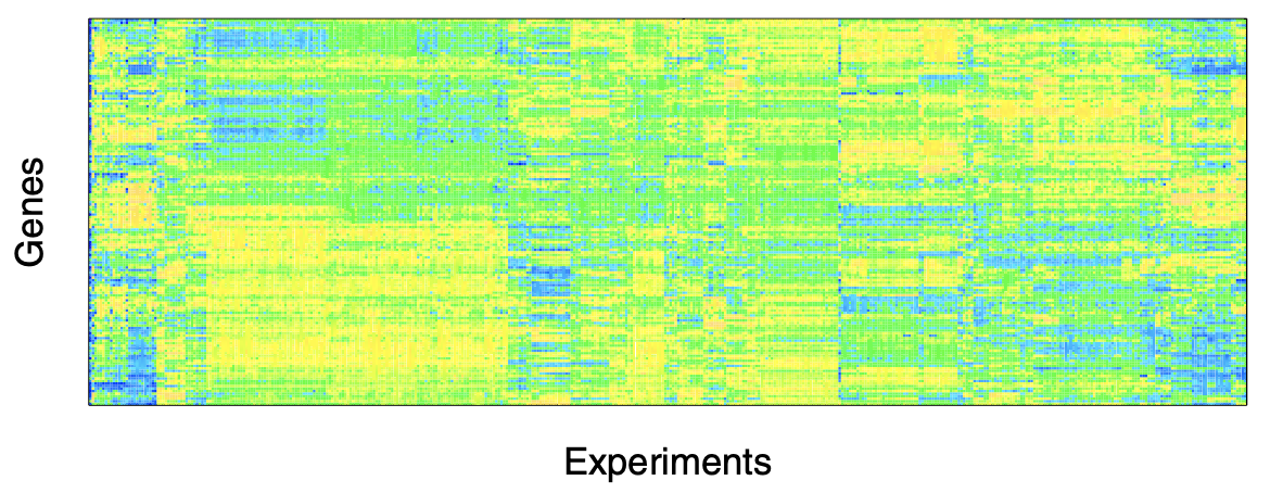
Fig. 222 Image representation of 445 microarray expression profiles collected for E. coli, under various conditions, for the 153 genes that are listed as known transcription factors (TF) in the RegulonDB, using blue-organge scale. [Kolaczyk 2009] database.
Challenge
A TF can actually be a target of another TF. And so direct correlation between measurements of a TF and a gene target may actually just be a reflection of the regulation of that TF by another TF. Sol: use partial correlation.
Methods and Results
Use three methods above, all use Fisher transformation for testing. See SAND pg.221-223
All methods have high precision and low recall. Faith et al. [SAND 140] have argued that the low recall is due primarily to limitations in both the number and the diversity of the expression profiles produced by the available experiments.
Takeaway: high precision model is still good for prediction purpose, though not good at recover old true labels (low recall).
Tomographic Inference
In tomographic network topology inference problems, measurements are available only at vertices that are somehow at the ‘exterior’ of the network, and it is necessary to infer the presence or absence of both edges and vertices in the ‘interior.’ Here ‘exterior’ and ‘interior’ are somewhat relative terms and generally are used simply to distinguish between vertices where it is and is not possible (or, at least, not convenient) to obtain measurements. For example, in computer networks, desktop and laptop computers are typical instances of ‘exterior’ vertices, while Internet routers to which we do not have access are effectively ‘interior’ vertices.
The problem of tomographic network topology inference is just one instance of what are more broadly referred to as problems of network tomography.
Introduction
Given
measurements at only a particular subset of vertices
Infer
topology of the rest
Challenge
For a given set of measurements, there are likely many network topologies that conceivably could have generated them
Without any further constraints on aspects like the number of internal vertices and edges, and the manner in which they connect to one another, we have no sensible way of choosing among these possible solutions.
The problem is thus an example of an ‘ill-posed inverse problem’ in mathematics – an inverse problem, in the sense of inverting the mapping from internal to external, and ill-posed, in the sense of that mapping being many-to-one.
In order to obtain useful solutions to such ill-posed problems, we impose assumptions on the internal structure.
Assumption
a key structural simplification has been the restriction to inference of networks in the form of trees.
Related fields
inference of phylogenies: to construct trees (i.e., phylogenies) from data, for the purpose of describing evolutionary relationships among biological species.
computer network analysis: to infer the tree formed by a set of paths along which traffic flows from a given origin Internet address to a set of destination addresses, including physical or logical topologies.
For Tree Topologies
Given a tree \(T=(V_T, E_T)\), let \(r \in V_T\) be its root, \(R \in V_T\) be its leaves, and \(V \setminus \left\{ \left\{ r \right\} \cup \left\{ R \right\}\right\}\) be the internal vertices. The edges \(E_T\) are often referred to as branches.
A binary three is also called a bifurcating tree, where each internal vertex has at most two children. We will restrict our attention here almost entirely to binary trees. Trees with more general branching structure can always be represented as binary trees and, indeed, methods for their inference can be built upon inferential methods for binary trees.
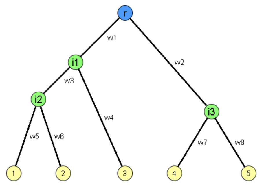
Fig. 223 Schematic representation of a binary tree. Measurements are available at the leaves 1, 2, 3, 4, and 5 (yellow). Other elements (possibly including the root \(r\)) are unknown.
The leaves \(R\) are known, but the internal vertices and the branches are not. The root \(r\) may or may not be known. We associate with each branch a weight \(w\), which we may or may not wish to infer.
For a set of \(N_\ell\) vertices, we have \(n\) independent and identically distributed observations of some random variables \(\left\{ X_1, X_2, \ldots, X_{N_\ell} \right\}\). Assume that these \(N_\ell\) vertices can be identified with the leaves \(R\) of a tree \(T\), we aim to find that tree \(T\) in the set \(\mathcal{T}_{N_\ell}\) of all binary trees with \(N_\ell\) labeled leaves that best explains the data, in some well-defined sense. If we have knowledge of a root \(r\), then the roots of the trees in \(\mathcal{T}_{N_\ell}\) will all be identified with \(r\). In some contexts we may also be interested in inferring a set of weights \(w\) for the branches in \(T\).
- Example (Binary multicast tree)
For instance, consider a binary multicast tree \(T\). There is a packet sending from root \(r\) to all \(N_\ell\) leaves. If the packet is ‘lost’ at an internal vertex, then all its descendants cannot receive the packet. Let \(X_i\) be binary variables, which is \(1\) if leave \(i\) receives the packet and \(0\) otherwise. We may send the packet for \(n\) times, obtain \(n\) binary vectors, and use them to infer the tree structure. Here are some properties of the tree which can be exploited in designing methods of inference:
For a subset \(U \in R\) of leaves, let \(a(U)\) be their closest common ancestor. If \(X_{a(U)} = 0\), then \(X_{u} = 0\) for all leaves \(u \in U\).
For an internal vertex \(v\), let \(C(v)\) be its children. If \(X_c = 1\) for at least one \(c \in C(v)\), then \(X_v = 1\).
- Example (Binary Phylogenetic tree)
Another example is DNA sequence. If we group DNA bases \(\left\{ A, G, C, T \right\}\) in pairs \(\left\{ A, G \right\}\) and \(\left\{ C, T \right\}\), i.e. by purines and pyrimidines respectively, and coded \(0\) and \(1\). We can then use an \(N_\ell\)-tuple of measurements to indicate whether each of \(N_\ell\) species being studied had a purine or pyrimidine at a given location in the genome. Repeat this for \(n\) different locations. Then we can form the notion of a tree-based evolutionary process generating sequence data at the leaves.
There are many methods for tomographic inference of tree topologies, which differ in
how the data are utilized (all or part)
criteria for assessing the merit of a candidate tree \(T \in \mathcal{T} _{N\ell}\) in describing the data
the number in which the space \(\mathcal{T} _{N_\ell}\) is searched in attempting to find a tree(s) best meeting this criteria.
Note that the space \(\mathcal{T} _{N_\ell}\) of (semi)labeled, rooted, binary trees is found to have \(\left(2 N_{l}-3\right) !! \approx \left(N_{l}-1\right)^{N_{l}-1}\) elements. Hence, exhaustive search is unrealistic and alternative approaches, based on greedy or randomized search algorithms, are utilized
maximum parsimony in phylogenetic inference, which seeks to construct a tree for data involving the minimum number of necessary evolutionary changes
branch-and-bound
Two popular classes of methods: hierarchical clustering-based, and likelihood-based. They both seek to exploit the supposition that, the closer two leaves are in the underlying tree, the more similar their observed characteristics (i.e., the measurements) will be.
the observed rate of shared losses of packets should be fairly indicative of how close two leaf vertices
two biological species are presumed to share more of their genome if they split from a common ancestor later in evolutionary time.
Hierarchical Clustering-based
Hierarchical clustering method can be used to the \(n \times N_\ell\) data matrix. Note that
traditional clustering methods aim to find cluster assignment, while here we want the hierarchical tree \(\hat{T}\).
the (dis)similarity measure can be customized, e.g. (true) shared loss, or genetic distance.
True, false and net shared loss in a multicast tree
There are two different types of shared loss between a pair of leaf vertices \(\left\{ j, k \right\}\) – termed ‘true’ and ‘false’ shared loss by Ratnasamy and McCanne [323].
The true shared losses are due to loss of packets on the path common to the vertices \(j\) and \(k\)
while the false shared losses are due to loss on the parts of paths following after the closest common ancestor, \(a(\left\{ j, k \right\})\).
For example, in the above tree,
true shared losses for the leaves 1 and 3 would be losses incurred on the path from \(r\) to the internal vertex \(i_1\);
false shared losses would refer to cases where packets were lost separately on the two paths from \(i_1\) to the vertices 1 and 3, respectively.
Since the net shared loss rate (i.e., the fraction of packets commonly lost to \(j\) and \(k\)) includes the contribution of both types of losses, it can be misleading to use this number as a similarity. Fortunately, it is possible to obtain information on the true loss rates from these net loss rates, through the use of a simple packet-loss model.
Here we introduce a Markov cascade process for multicast data. Consider the cascade process \(\left\{ X_j \right\}_{j \in V_T}\), assume \(X_r=1\). For each internal vertex \(k\), if \(X_k =0\) then \(X_j = 0\) for all child \(j \in C(k)\). If \(X_k = 1\), then we define
and hence define
\(A(k) = \prod_{j \succ k} \alpha_j\) to be the probability that a packet is transmitted from \(r\) to \(k\), where \(j \succ k\) indicates ancestral vertices \(j\) of \(k\) on the path from \(r\).
\(1 - A(a(\left\{ j, k \right\}))\) to be the true shared losses rate, i.e. shared loss due to loss of packets on the path common to the two leaf vertices \(j\) and \(k\).
\(R(k)\) to be the set of leaf vertices in \(R\) that are descendants of internal vertex \(k\)
\(\gamma(k)=\mathbb{P}\left(\cup_{j \in R(k)}\left\{X_{j}=1\right\}\right)\) be the probability that at least one of the leaves descended from \(k\) receive a packet. This can be estimated by \(n\) observations of \(\boldsymbol{x}_i\), using the relative frequency \(\hat{\gamma}(k)=(1 / n) \sum_{i=1}^{n}\left[\prod_{j \in R(k)} x_{ij}\right]\)
\(\gamma(U)=\mathbb{P}\left(\cup_{k \in U} \cup_{j \in R(k)}\left\{X_{j}=1\right\}\right)\) similarly, for an arbitrary set of vertices \(U\). In particular, if \(U = C(k)\), then \(\gamma(U) = \gamma(k)\).
Then, it is not difficult to show that for any \(U \subseteq C(k)\), we have
Therefore, we can first estimate \(\gamma(k)\) by \(\hat{\gamma}(k)\), then solve the above function to obtain \(\hat{A}(k)\) for all \(k \in V_T\). To build a agglomerative clustering tree, we can use the true shared losses rate \(1 - \hat{A}(a(\{j, k\}))\) as similarity measure. See [SAND 128] for consistency of the resulting estimator \(T\) for recovering a binary multicast tree \(T\), under the model assumptions.
Likelihood-based
We can specify a conditional density or PMF \(f(\boldsymbol{x} \vert T)\) for the \(N_\ell\)-length vector of random variables \(\boldsymbol{x} = [X_1, \ldots, X_{N_\ell}]\), given a tree-topology \(T\). If we assumed independence among the \(n\) observations, the likelihood has the form
and the MLE tree is simple \(\hat{T}_{ML} = \arg \max _{T \in \mathcal{T} _{N_\ell}} L(T)\). However, it is typically that there are parameters \(\boldsymbol{\theta}\) relating to the evolution of a tree \(T\). Hence, the likelihood has an integrated form
where \(f(\theta \vert T)\) is an appropriately defined distribution on \(\theta\), given \(T\). Depending on the nature of their integrands, the integrals may or may not lend themselves well to computational evaluation.
- Definition (Profile likelihood)
An alternative that can be more computationally tractable, or that can be used when we cannot or do not wish to specify a distribution \(f(\theta \vert T)\), is to define \(\hat{T}\) through maximization of a profile likelihood. Let
\[ L(T, \theta) =\prod_{i=1}^{n} f\left(\mathbf{x}_{i} \mid T, \theta\right) \]Then define
\[\begin{split}\begin{aligned} \hat{\theta}_{T} &= \arg \max _{\theta} L(T, \theta)\\ \widehat{T}_{PL}&=\arg \max _{T \in \mathscr{T}_{N_\ell}} L\left(T, \hat{\theta}_{T}\right) \\ \end{aligned}\end{split}\]where \(L\left(T, \hat{\theta}_{T}\right)\) is called the profile likelihood, and \(\widehat{T}_{PL}\) is called the maximum profile likelihood estimator.
For instance, for the multicast three model, \(\theta = \left\{ \alpha_j \right\}\), the profile likelihood is
where by chain rule factorization,
and \(pa(j)\) denotes the parent of \(j\) in \(T\).
The profile MLE is \(\widehat{T}_{P L}=\arg \max _{T \in \mathcal{T}_{N_{l}}} L\left(T, \hat{\alpha}_{T}\right)\), where \(\hat{\alpha}_{T}=\arg \max _{\alpha} L(T, \alpha)\). [SAND 128] prove its consistency under appropriate conditions.
Computation
Implementation of this estimator is non-trivial. For example, consider the estimation of \(\boldsymbol{\alpha}\), a parameter vector of potentially quite large dimension. An efficient, recursive estimation algorithm is proposed [SAND 71] using the relation
And recall that \(A(k)\) may be obtained from \(\gamma(k)\) and \(\gamma(k)\) can be estimated by frequencies. Although the resulting estimator \(\tilde{\alpha}_k\) is not strictly the maximum likelihood estimate, Caceres et al. [SAND 71] show that, when \(\alpha_k \in (0, 1)\) for all \(k\), we nevertheless have \(\tilde{\boldsymbol{\alpha}} = \hat{\boldsymbol{\alpha}}\) with high probability.
For the optimization of the profile likelihood \(L\left(T, \hat{\alpha}_{T}\right)\) for \(T \in \mathcal{T} _{N_\ell}\), if \(N_\ell\) is small (<5) we can use simulation for exhaustive search of \(\mathcal{T} _{N_\ell}\), else we can use greedy techniques or MCMC-based techniques.
In the phylogenetic tree example, we assume independence between measurements \(\boldsymbol{x}_i\) (e.g. between locations in the measured DNA sequence) and use Markov-like cascade model to capture the effects of evolution through time. By coding purines and pyrimidines as 0 and 1 respectively, we use a symmetric model of change between the two states of zero and one, in traversing from one end of a branch to the other, according to probability
parameterized by \(w_j\), the length of brach leading from \(k\) to \(j\), where \(j \in C(k)\).
The likelihood corresponding to this model is
where
Note that the summation (i.e. marginalization) is over all possible ways that the states zero or one can be assigned to the internal vertices of the tree \(T\), and is absent in the case of multicast data because of the hereditary constraints on the process \(\left\{ X_j \right\}j \in V_T\) (but still have multiple assignments??).
Computation
Likelihood: in general, the presence of such product-sum combinations can be problematic from a computational perspective. However, in this particular case, the likelihood can be calculated efficiently using a dynamic programming algorithm – the so-called pruning algorithm – proposed by Felsenstein [SAND 142]. Working recursively from the leaves towards the root, components of the likelihood are computed on sub-trees and combined in a clever fashion to yield the likelihoods on larger sub-trees containing them, until the likelihood for the entire tree is obtained.
Optimization in \((\widehat{T}, \hat{\mathbf{w}})\) is NP hard. In practice, a profile maximum likelihood method typically is used (??). See [SAND 143]. MCMC can also be pursued.
Summarizing Collections of Trees
All the above inference method output a single tree \(\hat{T}\), like a point estimate. Can we output a collection of trees, in the spirit of an interval estimate? In practice, such collections arise in various ways, such as
listing a number of trees of nearly maximum likelihood, rather than simply a single maximum-likelihood tree, or
from bootstrap re-sampling in an effort to assess the variability in an inferred tree, output \(\{\widehat{T}^{(b)}\}_{b=1}^{B}\), or
from MCMC sampling of an appropriate posterior distribution on \(\mathcal{T} _{N_\ell}\)
Given such a collection of trees, how can we usefully summarize the information therein? How they are similar or different?
For similarity, we can use consensus tree. A consensus tree is a single tree that aims to summarize the information in a collection of trees in a ‘representative’ manner. There are many methods to define such trees,
Margush and McMorris [SAND 268] defined \(M_\ell\)-trees indexed by \(\ell \in [0.5, 1]\), which contains all groups of leaves \(U \subseteq R\) that occur in more than a fraction \(\ell\) of the trees in a collection.
\(\ell=1\), it is called strict consensus tree
\(\ell=0.5\), it is called majority-rule consensus tree
additional information can be added to a consensus tree in the form of branch weights
For differences, there are various notions of distance between pairs of trees
symmetric difference works by counting branches.
nearest-neighbor interchange (NNI) counts the number of swaps of adjacent branches that must be made to transform one tree into the other (computationally daunting)
both are metrics
Relationships: if we define a median tree in a collection to be a tree \(T\) whose total distance – based on the symmetric difference – to all other trees is a minimum, then this tree is equivalent to the majority-rule tree, when the number of trees \(t\) in the collection is odd [SAND 21].
More
More examples
link prediction / association networks
inferring networks from so-called co-occurrence data, e.g. telecommunications and genetics [SAND 318, 319]
protein complexes [SAND 343]
inferring networks with links defined according to the dynamic interactions of elements in a system (e.g., such as of information passing between neurons firing in sequence). [SAND 355]
tomographic inference
infer coalescent trees, which have to do with the evolution of genes within a population (i.e., below the level of species). See Felsenstein [141, Ch. 26].
More measurements
association networks
Spearman rank correlation and partial correlation might be used as robust alternatives to Pearson correlation [350.sec.3.9], [110]
Or a measure capable of summarizing nonlinear association, such as mutual information [140]
computer networks
mean delay, see the sandwich probing in case study 7.4.5.
Open problems
basic questions of consistency, consensus, robustness, beyond trees?
how to best characterize the merit of partially accurate estimates \(\hat{G}\)? e.g. focusing on the accuracy with which small subgraphs (e.g., network motifs) or paths are recovered.