Sampling and Estimation¶

Like other statistical data, we usually only observe a sample from a larger underlying graph. We introduce sampling and estimation in graphs.

Sampling¶

Graph sampling designs are somewhat distinct from typical sampling designs in non-network contexts, in that there are effectively two inter-related sets $V$ and $E$ of units being sampled. Often these designs can be characterized as having two stages:

a selection stage, among one set (e.g. vertices)
an observation stage, among the other or both

It’s also important to discuss the inclusion probabilities of a vertex and an edge in each sampling design, denoted $\pi_i$ for vertex $i \in E$ and $\pi_{(i, j)}$ for edge $(i,j) \in V^{(2)}$, where $V^{(2)}$ is the set of all unordered pairs of vertices.

Induced Subgraph Sampling¶

The two stages are

Select a simple random sample of $n$ vertices $V^{*}=\left\{i_{1}, \ldots, i_{n}\right\}$ from $V$ without replacement
Observe a set $S^*$ of edges in their induced subgraphs: for $n(n-1)$ pairs of $(i, j)$ for $i,j \in V^*$, check whether $(i,j)\in E$.

For instance, in social networks, we an sample a group of individuals, and then ask their relation or some measure of contact, e.g. friendship, likes or dislike.

The inclusion probabilities are uniformly equal to

\[\begin{split}\begin{aligned} \pi_{i}&= \mathbb{P}\left( v_i \text{ is selected} \right) \\ &= \frac{n}{N_v} \\ \pi_{(i,j)}&= \mathbb{P}\left( \text{both $v_i$ and $v_j$ are selected} \right) \\ &= \mathbb{P}\left( \text{$v_i$ is selected} \right) \mathbb{P}\left( \text{$v_j$ is selected} \mid \text{$v_i$ is selected} \right)\\ &= \frac{n}{N_v} \cdot \frac{n-1}{N_v - 1} \quad \because \text{without replacement} \end{aligned}\end{split}\]

Note that $N_v$ is necessary to compute these probabilities.

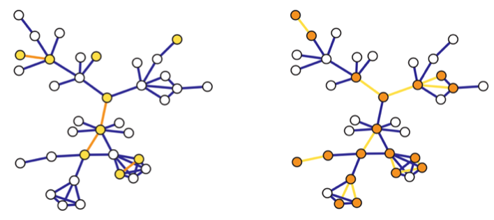
Fig. 207 Induced (left) and incident (right) subgraph sampling. Selected vertices/edges are shown in yellow, while observed edges/vertices are shown in orange.¶

Incident Subgraph Sampling¶

Complementary to induced subgraph sampling is incident subgraph sampling. Instead of selecting $n$ vertices in the initial stage, $n$ edges are selected:

Select a simple random sample $E^*$ of $n$ edges from $E$ without replacement
All vertices incident to the selected edges are then observed, thus providing $V^*$.

For instance, we sample email correspondence from a database, and observe the sender and receiver.

Inclusion probabilities:

\[\begin{split}\begin{aligned} \pi_{(i, j)} &= \frac{n}{N_e} \\ \pi_i&= 1-\mathbb{P}(\text{no edge incident to $v_i$ is selected}) \\ &=\left\{\begin{array}{ll}\frac{\binom{N_e - d_i}{n}}{\binom{N_e}{n}} & \text { if } n \leq N_{e}-d_{i} \\ 1, & \text { if } n>N_{e}-d_{i}\end{array}\right. \\ \end{aligned}\end{split}\]

Hence, in incident subgraph sampling, while the edges are included in the sample graph $G^*$ with equal probability, the vertices are included with unequal probabilities depending on their degrees.

Note that $N_e$ and $d_i$ are necessary to compute the inclusion probabilities. In the example of sampling email correspondence graph, this would require having access to marginal summaries of the total number of emails (say, in a given month) as well as the number of emails in which a given sender had participated.

Star Sampling¶

The first stage selects vertices like in induced subgraph sampling, but in the second stage, as its name suggests, we sample all edges incident to the selected vertices, as well as the new vertices on the other end.

Select a simple random sample $V_0^*$ from $V$ without replacement
For each $v \in V^*$,
- observe all edges incident to $v$, yielding $E^*$.
- also observe its neighbors, together with $V_0^*$ yielding $V^*$

More precisely, this is called labeled star sampling. In unlabeled star sampling, the resulting graph is $G^* = (V_0^*, E^*)$. In the latter case, we focus on some particular characteristics (e.g. degrees), so we don’t need the vertices on the other end.

For instance, in co-authorship graph, randomly sampling records of $n$ authors and recording the total number of co-authors of each author would correspond to unlabeled star sampling; if not only the number but the identities of the co-authors are recorded, this would correspond to labeled star sampling.

The inclusion probabilities are

\[\begin{split}\begin{aligned} \pi_{(i, j)} &= \mathbb{P}\left( \text{neither $i$ nor $j$ are sampled} \right)\\ &= 1- \frac{\binom{N_v-2}{n}}{\binom{N_v}{n}} \\ \pi_ i &= \frac{n}{N_v} \quad \text{unlabeled case} \\ \pi_ i &= \sum_{L \subseteq N[i]}(-1)^{|L|+1} \mathbb{P}(L) \quad \text{labeled case} \\ \end{aligned}\end{split}\]

where

$N[i]$ is the union of vertex $i$ and the its immediate neighbors
$\mathbb{P}\left( L \right) = \frac{\binom{N_v - \left\vert L \right\vert}{n - \left\vert L \right\vert} }{\binom{N_v}{n} }$ is the probability that $L \subseteq V_0^*$. ($n > \left\vert L \right\vert$??)

Snowball sampling¶

In star sampling we only look at the immediate neighborhood. We can extends it to up to the $K$-th order neighbors, which is snowball sampling. In short, a $K$-stage snowball sampling is

select a simple random sample $V_0^*$ from $V$ without replacement
for each $k = 1, \ldots , K$, observe a $k$-th order neighbors, add them to $V^*$ (excluding repeated vertices), and add their incident edges to $E^*$.

Formally, let $N(S)$ be the set of all neighbors of vertices in a set $S$. After we initialize $V_0^*$, we add vertices, for $k=1, \ldots, K$

$V_k^* = N(V_{k-1}^*)\cap \bar{V}_0^* \cap \ldots \cap \bar{V}_{k-1}^*$, called the $k$-th wave.

A termination condition is $V_k = \emptyset$. The final graph $G^*$ consists of the vertices in $V^* = V_0^* \cup V_1 ^* \cup \ldots \cup V_K^*$ and their incident edges.

Unfortunately, although not surprisingly, inclusion probabilities for snowball sampling become increasingly intractable to calculate after the one-stage level corresponding to star sampling.

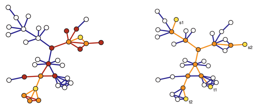
Fig. 208 Two-stage snowball sampling (left) where $V_0^*$ in yellow, $V_1^*$ in orange, and $V_2^*$ in red. Traceroute sampling (right) for sources $\left\{ s_1, s_2 \right\}$ and targets $\left\{ t_1, t_2 \right\}$ in yellow, observed vertices and edges in orange.¶

Link Tracing¶

Many of the other sampling designs fall under link tracing designs: after some selection of an initial sample, some subset of the edges (‘links’) from vertices in this sample are traced to additional vertices.

Snowball sampling is a special case of link tracing, in that all edges are observed. Sometimes this is not feasible, for example, in sampling social contact networks, it may be that individuals are unaware of or cannot recall all of their contacts, or that they do not wish to divulge some of them.

We introduce traceroute sampling.

select a random sample $S=\left\{s_{1}, \ldots, s_{n_{s}}\right\}$ of vertices as sources from $V$, and another random sample $T=\left\{t_{1}, \ldots, t_{n_{t}}\right\}$ of vertices as targets from $V \setminus S$.
For each pair $(s_i, t_j) \in S \times T$, sample a $s_i$-$t_j$ path. Observe all vertices and edges in the path, whose union yielding $G^* = (V^*, E^*)$.

To find the inclusion probabilities, we assume that the paths are shortest paths w.r.t. some set of edge weights. Dall’Asta et al. [SAND 107] find the probabilities are

\[\begin{split}\begin{aligned} \pi_{i} &\approx 1-\left(1-\rho_{s}-\rho_{t}\right) \exp \left(-\rho_{s} \rho_{t} b_{i}\right) \\ \tau_{\{i, j\}} &\approx 1-\exp \left(-\rho_{s} \rho_{t} b_{i, j}\right) \end{aligned}\end{split}\]

where

$b_i$ is the vertex betweenness centrality of vertex $i$
$b_{i, j}$ is the edge betweenness centrality of edge $(i, j)$
$\rho_{s} = \frac{n_s}{N_v} , \rho_t = \frac{n_t}{N_v}$ are the source ant target sampling fractions respectively

We see that the unequal probabilities varies with betweenness centrality $b_i$ and $b_{i, j}$. Though they are not calculable, they lend interesting insight into the nature of this sampling design, to be introduced later.

Estimation¶

(Review the estimation of total section)

With appropriate choice of population $U$ and unit values $y_i$ for $i \in U$, many of the quantities $\eta(G)$ of graph $G$, e.g. average degree, $N_e$, or even centrality, can be written in a form of population total $\sum_{i \in U} y_i$, as introduced below.

To estimate the total from a sampled graph $G^* = (V^*, E^*)$ where $V^* \subseteq V, E^* \subseteq E$, we can use generalization of the Horvitz-Thompson estimator.

Types¶

Many estimation problems can be classified to totals over some order of vertex set $V^(k)$.

Totals on Vertex¶

Let $U=V$, we can define $y_i$ according to the total we are interested.

average degree: let $y_i = d_i$, then the average degree $\bar{d}$ equals the population total $\sum_{i \in V} d_i$ divided by $N_v$
proportion of special vertices: let $y_i = \mathbb{I} \left\{ v_i \text{ has some property} \right\}$, then the proportion of such special vertices equals the population total $\sum_{i \in V} 1$ divided by $N_v$. For instance, proportion of gene responsible for the growth of an organism.

Given a sample of vertices $V^* \subseteq V$, the Horvitz-Thompson estimator for vertex totals takes the form

\[ \hat{\tau}_{\pi}=\sum_{i \in V^{*}} \frac{y_{i}}{\pi_{i}} \]

Note that

in some sampling design, the graph structure will be irrelevant for estimating a vertex total, e.g. when the graph structure is irrelevant to $y$ and vertices are sampled through simple random sampling without replacement. $\pi_i$ can be computed in the conventional way.
on the other hand, the graph structure matters, e.g. in snowball sampling the structure determines $V^*$ and hence the calculation of $\pi_i$.

Totals on Vertex Pairs¶

Now we are interested in $U = V^{(2)}$, the total is

\[ \tau=\sum_{(i, j) \in V^{(2)}} y_{i j} \]

number of edges: let $y_{(i, j)} = \mathbb{I} \left\{ (i,j) \in E \right\}$, then the number of edges $N_e$ is given by the total.
betweenness centrality: let $y_{(i,j)} = \mathbb{I} \left\{ v \in P(i,j) \right\}$ where $P(i,j)$ is the shortest path between $i$ and $j$, and $y_{(i, j)} = 1$ if vertex $v$ is in this shortest path. If all shortest paths are unique, then the betweenness centrality $c_{bet}(v)$ of a vertex $v \in V$ is given by the total, which counts how many shortest paths going through $k$.
number of homogeneous vertices: let $y_{(i,j)} = \mathbb{I} \left\{ \text{both } i \text{ and } j \text{ have some properties} \right\}$
average of some (dis)similarity value between vertex: let $y_{(i,j)} = s(i, j)$ and then divide the total by $N_e$.

The Horvitz-Thompson estimator takes the form

\[ \hat{\tau}_{\pi}=\sum_{(i, j) \in V^{*(2)}} \frac{y_{i j}}{\pi_{i j}} \]

If $y_{ij} \ne 0$ iff $(i, j) \in E$, then

vertex pairs total $\tau$ equals to an edge total
summation in the estimator $\hat{\tau}$ is taken over $E^*$,
the inclusion probability $\pi_{ij}$ is just the edge inclusion probability $\pi_{(i, j)}$, which equals
- $\frac{n(n-1)}{N_v (N_v - 1)}$ under induced graph sampling with simple random sampling without replacement in stage 1
- $\frac{1}{p^2}$ under induced graph sampling with Bernoulli sampling with probability $p$ in stage 1

The variance of the above estimator, generalized from that for conventional Horvitz-Thompson estimator, is given by

\[ \mathbb{V}\left(\hat{\tau}_{\pi}\right)=\sum_{(i, j) \in V^{(2)}} \sum_{(k, l) \in V^{(2)}} y_{i j} y_{k l}\left(\frac{\pi_{i j k l}}{\pi_{i j} \pi_{k l}}-1\right) \]

where $\pi_{ijkl}$ is the probability that units $(i,j)$ and $(k,l)$ are both included in the sample, and $\pi_{ijkl} = \pi_{ij}$ for convenience when $(i,j) = (k, l)$. Note that there can be $1 \le r \le 4$ different vertices among $i,j,k,l$. The corresponding unbiased estimate of this variance is given by

\[ \widehat{\mathbb{V}}\left(\hat{\tau}_{\pi}\right)=\sum_{(i, j) \in V^{*(2)}} \sum_{(k, l) \in V^{*(2)}} y_{i j} y_{k l}\left(\frac{1}{\pi_{i j} \pi_{k l}}-\frac{1}{\pi_{i j k l}}\right) \]

Note that these quantities can become increasingly complicated to compute under some sampling designs, since it is necessary to be able to evaluate probabilities $\pi_{ijkl}$ for $1 \le r \le 4$. See Example 5.4 in SAND pg.139 for $p_r$ in induced graph sampling and estimation of $N_e$. Results are shown below.

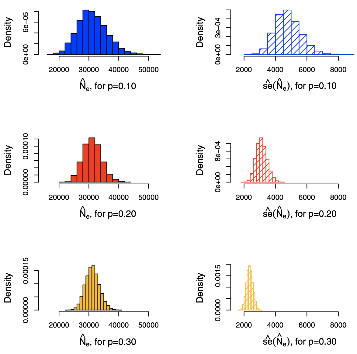
Fig. 209 Histograms of estimates $\hat{N}_e$ of $N_e$ = 31201 and its estimated standard errors (right), under induced subgraph sampling, with Bernoulli sampling of vertices using $p=0.1, 0.2, 0.3$ based on 10000 trials. [Kolaczyk 2009]¶

Totals of Higher Order¶

The expressions for higher order cases are more complicated. We introduce the case of triples, where $U = V^{(3)}$ and $\tau=\sum_{(i, j, k) \in V^{(3)}} y_{i j k}$. The sample Horvitz-Thompson estimator is

\[ \hat{\tau}_{\pi}=\sum_{(i, j, k) \in V^{*(3)}} \frac{y_{i j k}}{\pi_{i j k}} \]

The expressions for variance and estimated variance follow in a like manner.

We see an example of estimating transitivity. Recall that

\[ \operatorname{clus}_{T}(G)=\frac{3 \tau_{\Delta}(G)}{\tau_{\wedge}(G)} \]

where

$\tau_{\Delta}(G)=\frac{1}{3} \sum_{v \in V} \tau_{\Delta}(v)$ is the number of triangles in the graph
$\tau_{\wedge}(G)=\sum_{v \in V} \tau_{\wedge}(v)$ is the number of connected triples in the graph

This quantity can be re-expressed in the form

\[ \operatorname{clus}_{T}(G)=\frac{3 \tau_{\Delta}(G)}{\tau_{\wedge} ^ +(G) + 3 \tau_{\Delta}(G)} \]

where $\tau_{\wedge} ^ +(G) = \tau_{\wedge}(G) - 3 \tau_{\Delta}(G)$ is the number of vertex triples that are connected by exactly two edges. Then both $\tau_{\Delta}(G)$ and $\tau_{\wedge}^+(G)$ can becomputed as a total $\sum_{(i,j,k) \in V^{(3)} }y_{ijk}$ by setting, respectively,

$y_{ijk} = a_{ij}a_{jk}a_{ki}$
$y_{i j k}=a_{i j} a_{j k}\left(1-a_{k i}\right)+a_{i j}\left(1-a_{j k}\right) a_{k i}+\left(1-a_{i j}\right) a_{j k} a_{k i}$

where $a_{ij}$ is the $ij$-th entry in the adjacency matrix.

If we use induced subgraph sampling with Bernoulli sampling of vertices with probability $p$ to obtain a sample $G^* = (V^*, E^*)$, then $\pi_{ijk} = p^{-3}$, and hence

\[ \hat{\tau}_{\Delta}(G) =\sum_{(i, j, k) \in V^{*(3)}} \frac{y_{i j k}}{\pi_{i j k}} = p^{-3} \sum_{(i, j, k) \in V^{*(3)}}y_{i j k} = p^{-3} \tau_{\Delta}(G^*) \]

and similarly $\hat{\tau}_{\wedge}^+(G) = p^{-3}\tau_{\wedge}^+(G^*)$.

We can then substitute these two values to obtain a plug-in estimator of transitivity $\operatorname{clus}_T (G)$. Note that the coefficient $p^{-3}$ cancel out, hence $\widehat{\operatorname{clus}}_T (G) = \operatorname{clus} _T (G^*)$.

Summary¶

There are three conditions to make the estimation feasible

the graph summary statistic $\eta(G)$ must be expressed in terms of totals
the values $y$ must be either observed or obtainable from the available measurements
the inclusion probabilities $\pi$ must be computable for the sampling design

But it is not always the case that all three elements are present at the same time. As the first example shown below.

In fact, many estimation problems can be viewed as species problems.

average degree: how many (distinct) edges for each observed vertex?
$N_e$ via link tracing: how many distinct edges on multiple paths?

Examples¶

Average Degree¶

We will see estimating average degree using two different sampling designs.

First consider unlabeled star sampling. Let the sampled graph be $G^*_{star} = (V^*_{star}, E^*_{star})$. The average degree is a rescaling of vertex total

\[ \hat{\mu}_{star} = \frac{\hat{\tau}_{star}}{N_v} \quad \text{where} \quad \hat{\tau}_{star} = \sum_{i \in V_{star}^*} \frac{d_i}{n/N_v} \]

Note that $d_i$ is observed.

On the other hand, under induced subgraph sampling, we do not observe $d_i$, but only a number $d_i^* \le d_i$ for each $i \in V_{indu}^*$. As a result, $\tau$ is not amenable to Horvitz-Thompson estimation methods as a vertex total.

However, we can use the relation $\mu = \frac{2N_e}{N_v}$, which shows an alternative way by estimating $N_e$. As introduced in total on vertex pairs above, with inclusion probability $\pi_{ij}= \frac{n(n-1)}{N_v (N_v - 1)}$, we have

\[ \hat{N}_{e, indu}=\sum_{(i, j) \in E_{indu}^{*}} \frac{1}{\pi_{ij}}=N_{e, indu}^{*} \cdot \frac{N_{v}\left(N_{v}-1\right)}{n(n-1)} \]

which gives the unbiased estimator

\[ \hat{\mu} _{indu} = \frac{2 \hat{N}_{e, indu}}{N_v} \]

for $\mu$

We can then compare these two estimator. Some re-writing gives

\[ \hat{\mu}_{star} = \frac{2N_{e, star}^*}{n} \quad \hat{\mu}_{I S}=\frac{2 N_{e, indu}^{*}}{n} \cdot \frac{N_{v}-1}{n-1} \]

Hence under star sampling, it simply use the relation $\bar{d} = \frac{2N_e}{N_v}$ to the sample. In contrast, under induced subgraph sampling, the analogous result (sample average degree) is scaled up by the factor $\frac{N_v - 1}{n-1}$ to account for $d_{i, indu}^* \le d_i$.

Hidden Population Size¶

The term ‘hidden population’ generally refers to one in which the individuals do not wish to expose themselves to view. For example, humans of socially sensitive status, such as illegal drug usage or prostitution. Two issues:

they will not be inclined to disclose themselves
their population is small

Frank and Snijders [SAND 154] describe how snowball sampling may be used for this problem, using the idea that mimics capture-recapture methods.

Let

$V$ be the set of all members of the hidden population
$G = (V,E)$ be a directed graph associated with that population, in which an arc from vertex $i$ to vertex $j$ indicates that, if asked, individual $i$ would mention individual $j$ as a member of the hidden population (there are some concerns of trust, veracity etc). We want to estimate $N_v$.
$G^*$ be a subgraph of $G$, where the vertices $V^* = V_0^* \cup V_1 ^*$ are obtained through a one-wave snowball sample, with the initial sample $V_0^*$ selected through Bernoulli sampling $Z_i \sim \operatorname{Ber}(p_0)$ from $V$, where the sampling rate $p_0$ is unknown. We have three random variables
- $N_v ^* = \left\vert V_0^* \right\vert$ be the size of the initial sample
- $M_1$ be the number of arcs $(i, j)$ in $V_0^*$ ($i \in V_0^*$ and $j \in V_0^*$)
- $M_2$ be the number of arcs pointing from $i \in V_0^*$ to $j \in V_1^*$ ($i \in V_0^*$ but $j \notin V_0^*$)

Out estimator of $N_v$ will be derived using the method-of-moments. We first find the expectation of the three variables.

\[\begin{split} \begin{array}{l} \mathbb{E}(N_v ^*)=\mathbb{E}\left(\sum_{i} Z_{i}\right)=N_{v} p_{0} \\ \mathbb{E}\left(M_{1}\right)=\mathbb{E}\left(\sum_{i \neq j} Z_{i} Z_{j} A_{i j}\right)=\left(N_{e}-N_{v}\right) p_{0}^{2} \\ \mathbb{E}\left(M_{2}\right)=\mathbb{E}\left(\sum_{i \neq j} Z_{i}\left(1-Z_{j}\right) A_{i j}\right)=\left(N_{e}-N_{v}\right) p_{0}\left(1-p_{0}\right) \end{array} \end{split}\]

Setting the left-hand sides of these equations equal to their observed counterparts, say $n_v ^*, m_1$ and $m_2$ gives

\[\begin{split}\begin{aligned} \hat{p}_0&= \frac{m_1 + m_2}{m_1} \\ \widehat{N_v} &= \frac{1}{\hat{p}_0} n_v ^*\\ \end{aligned}\end{split}\]

In other words, the number of individuals observed initially is inflated by an estimate $\hat{p}_0$ of the sampling rate, where that estimate reflects the relative number of arcs from individuals in the initial sample that point inwards among themselves.

To find the variance this estimator, we use the jackknife principle. Let $\widehat{N}_{v}^{(-i)}$ be the estimate of $N_v$ obtained by removing $i \in V_0^*$ and $j \in V_1^*$ that has only one edge $(i, j)$ adjacent to it, and let $\bar{\widehat{N}}_v$ be their average, then

\[ \widehat{\mathbb{V}}_{J}\left(\widehat{N}_{v}\right)=\frac{n-2}{2 n} \sum_{i \in V_{0}^{*}}\left(\widehat{N}_{v}^{(-i)}-\bar{\widehat{N}}_v\right)^{2} \]

Graph Size via Link Tracing¶

We can estimate graph size via link tracing (traceroute sampling).

Let $V_{(-j)}^{*}$ denote the number of vertices discovered on sampled paths to targets other than $t_{j},$ and define $\delta_{j}= \mathbb{I} \left\{t_{j} \notin V_{(-j)}^{*}\right\}$ to be the indicator of the event that target $t_{j}$ is not ‘discovered’ on sampled paths to any other target. Write the total number of such targets as $X=\sum_{j} \delta_{j}$. We want to find $\mathbb{E} [X]$, i.e. the average tendency of targets to be missed by other paths.

Given a set of pre-selected source nodes $S=\left\{s_{1}, \ldots, s_{n_{s}}\right\}$ (chosen either randomly or not), if the target nodes in $T=\left\{t_{1}, \ldots, t_{n_{t}}\right\}$ are chosen by simple random sampling without replacement from $V \backslash S$, the probability that target $t_{j}$ is not discovered on the paths to other targets is given by

\[ \begin{align*} \mathbb{P}\left(\delta_{j}=1 \mid V_{(-j)}^{*}\right)=\frac{N_{v}-N_{(-j)}^{*}}{N_{v}-n_{s}-(n_{t}-1)} \end{align*} \]

where $N_{(-j)}^{*}=\left|V_{(-j)}^{*}\right|$. Note that, by symmetry under simple random sampling for $t_j \in T$, the expectation $\mathbb{E}[N_{(-j)}^{*}]$ is the same for all $j .$ We denote this quantity by $\mathbb{E}[N_{(-)}^{*}]$ and, as a result, we obtain

\[ \begin{align*} \mathbb{E}[X]=\sum_{j=1}^{n_{t}} \mathbb{P}\left(\delta_{j}=1 \mid V_{(-j)}^{*}\right)=\frac{n_{t}\left[N_{v}-\mathbb{E}[N_{(-)}^{*}]\right]}{N_{v}-n_{s}-n_{t}+1} \end{align*} \]

The only unknown quantity in this equation is $N_v$, while others can be pre-set or estimated. Rewriting this equation we have

\[ N_{v}=\frac{n_{t} \mathbb{E}[N_{(-)}^{*}]-\left(n_{s}+n_{t}-1\right) \mathbb{E}[X]}{n_{t}-\mathbb{E}[X]} \]

Hence, we have a method-of-moments estimator for $N_v$. In a run of link tracing, an unbiased estimator of $\mathbb{E} [X]$ is the $X$ itself, and that of $\mathbb{E}[N_{(-)}^{*}]$ is the average of $N_{(-i)}^*$. However, if $X = n_t$, then RHS denominator is not well defined.

To solve this, under a slight variation of this idea and ignoring trivial terms and factors, Viger et al. [SAND 388] arrive at an estimator of the form

\[ \hat{N}_{v}=\left(n_{S}+n_{t}\right)+\frac{N_{v}^{*}-\left(n_{S}+n_{t}\right)}{1-w^{*}} \]

where $w^{*}=X /\left(n_{t}+1\right)$, hence the denominator can be viewed as the average tendency of targets to be discovered by other paths. A simple estimate of the variance of this by delta-method is

\[ \widehat{\mathbb{V}}\left(\hat{N}_{v}\right) \approx \frac{\left(N_{v}^{*}-n_{S}-n_{t}\right)^{2} w^{*}}{\left(1-w^{*}\right)^{3} n_{t}} \]

Issues¶

Usually, we want to estimate some characteristic $\eta(G)$ of a graph $G$ through sampled subgraph $G^*$. Some sampling designs give biased characteristic $\eta(G^*) \ne \eta(G)$ but can be adjusted, like the average degree example above. But if $\eta$ is more involved, this is no trivial. For instance, many sampling designs induce degree distribution unrepresentative of the true underlying degree distribution [SAND pg.150].

Let $f_d$ and $f_d^*$ be the true and observed frequencies of degree $d$ nodes in $G$ and $G^*$, respectively. Frank [SAND 153] shows under induced subgraph sampling,

\[ \mathbb{E}\left(f_{d}^{*}\right)=\sum_{d^{\prime}=0}^{N_{v}-1} P\left(d, d^{\prime}\right) f_{d^{\prime}}, \quad \text{where} P\left(d, d^{\prime}\right)=\frac{\binom{d^{\prime}}{d}\binom{N_{v}-1-d^{\prime}}{n-1-d}}{\binom{N_{v}-1}{n-1}} \]

where $\binom{n}{k} = 0$ if $k >n$. In principle, to find $f_d$, we can substitute $f_d^*$ to LHS, and obtain a system of equations for unknowns $(f_0, \ldots, f_N)$. But since $n < N$, this is system of equations is under-determined unless it is known that $d_\max < n$. Even this is true, the solution is not guaranteed to be non-negative, and the variance of this estimator would not be easy to derive.

Other issues

analysis of non-traditional sampling designs (e.g., particularly adaptive designs)
the estimation of quantities not easily expressed as totals (e.g., degree distribution exponents)
the incorporation of effects of sampling error and missingness

Data Science Handbook

Sampling and Estimation¶

Sampling¶

Induced Subgraph Sampling¶

Incident Subgraph Sampling¶

Star Sampling¶

Snowball sampling¶

Link Tracing¶

Estimation¶

Types¶

Totals on Vertex¶

Totals on Vertex Pairs¶

Totals of Higher Order¶

Summary¶

Examples¶

Average Degree¶

Hidden Population Size¶

Graph Size via Link Tracing¶

Issues¶