Topic Models
Topic models are generative “mixture” models for documents.
The data we have in hand are \(D\) documents. Each document \(d\) has \(n_d\) words. Topic model assumes that there is a topic \(t_d\) for each document, which is latent, unobservable.
Generative Process
Now we generate the \(D\) documents.
Assumptions
For a document \(d\),
Its topics \(t_d\) is unknown. Suppose there are \(k_t\) kinds of possible topics, then \(t_d\) can be drawn from a multinomial distribution parameterized by \(\boldsymbol{\alpha} \in \mathbb{R} ^{k_t}\).
\[t_d \sim \operatorname{Multinomial}(\boldsymbol{\alpha}) \]The words \(w_1, \ldots, w_{n_d}\) are i.i.d. drawn from multinomial distribution of \(k_w\) kinds of words, parameterized by \(\boldsymbol{\beta} \in \mathbb{R} ^{k_w}\). The words distribution can be determined by the document topic \(t_d\), i.e. \(\boldsymbol{\beta} _{t_d}\), hence
\[w \sim \operatorname{Multinomial}(\boldsymbol{\beta}_{t_d})\]We can impose prior distributions on \(\boldsymbol{\beta}\) and \(\boldsymbol{\alpha}\), which are Dirichlet distributions, parameterized by \(\boldsymbol{\eta}\) and \(\boldsymbol{\theta}\) respectively.
\[\begin{split}\begin{aligned} \boldsymbol{\beta} &\sim \operatorname{Dirichlet}(\boldsymbol{\eta} ) \\ \boldsymbol{\alpha} &\sim \operatorname{Dirichlet}(\boldsymbol{\theta} ) \end{aligned}\end{split}\]
Hence, to generate \(D\) documents, each with \(\sum_{d=1}^D n_d\) number of random words, the steps are
For each document \(d=1, \ldots, D\)
Draw a topic vector \(\boldsymbol{\alpha} \sim \operatorname{Dirichlet}(\boldsymbol{\theta})\)
Draw \(k_t\) vectors \(\boldsymbol{\beta}, \ldots, \boldsymbol{\beta}_{k_t} \sim \operatorname{Dirichlet}(\boldsymbol{\eta})\)
Generate words: for \(1, \ldots, n_d\)
Draw a topic \(t\sim \operatorname{Multinomial}(\boldsymbol{\alpha} )\)
Draw a word \(w\sim \operatorname{Multinomial}(\boldsymbol{\beta}_{t})\)
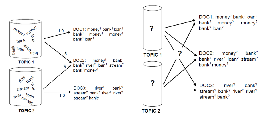
Fig. 142 Topic model (generation vs estimation)
Estimation
In a document of words \(w_1, \ldots, w_{n_d}\), we want to estimate the underlying word distribution \(\boldsymbol{\beta} = \left[ \beta_1, \ldots, \beta_{k_w} \right]\). A simple approach is to use maximum likelihood
For some word labeled \(m\), this is
Other variables include \(t\)’s, \(\boldsymbol{\alpha}\)’s, which can be estimated by Expectation Maximization (EM) algorithm and sampling-based methods (MCMC and Gibbs sampling)
The learned results are like
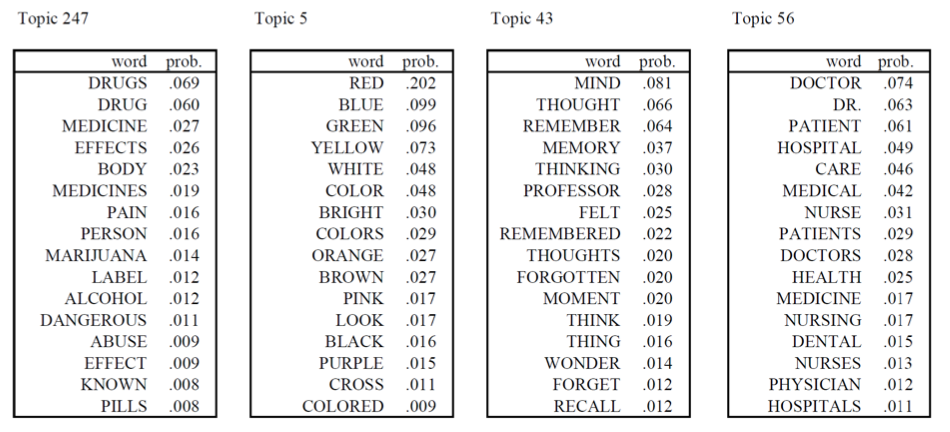
Fig. 143 Learned words distribution parameters \(\boldsymbol{\beta} _t\) by topics [Steyvers & Griffiths, 2007]