Exponential Families
One-parameter Exponential Family
Definition
Consider a random variable \(Y\) with probability density function parameterized by \(\theta \in \mathbb{R}\). If its PDF can be written in the form
where
\(b(\theta)\) is some function of \(\theta\)
\(f_0(x)\) involves only \(x\), no \(\theta\)
then we call there PDF from one-parameter exponential family, where “one” means \(\theta \in \mathbb{R} ^1\).
Some examples include
Normal with known variance \(\sigma^2\), parameterized by \(\mu\)
\[ f(x)=\frac{1}{\sqrt{2\pi\sigma^{2}}}\exp(-\frac{1}{2\sigma^{2}}(x^{2}-2\mu x+\mu^{2}))=\underbrace{\frac{1}{\sqrt{2\pi\sigma^{2}}}\exp\left(-\frac{x^{2}}{2\sigma^{2}}\right)}_{\theta}{f_{0}(x)}\exp\left(x\underbrace{\frac{\mu}{\sigma^{2}}}_{\theta}-\frac{\mu^{2}}{2\sigma^{2}}\right) \]Bernoulli parameterized by \(p\)
\[ \mathbb{P} (X=x)=p^{x}(1-p)^{1-x}=\exp(x\underbrace{\ln\frac{p}{1-p}}_{\theta}+\ln(1-p)) \]Binomial parameterized by \(p\)
\[ \mathbb{P} (X=x)=\binom{n}{x} p^{x}(1-p)^{n-x}= \binom{n}{x} \exp(x\underbrace{\ln\frac{p}{1-p}}_{\theta}+n\ln(1-p)) \]Poisson parameterized by \(\mu\)
\[ \mathbb{P} (X=x)=\frac{e^{-\mu}\mu^{x}}{x!}=\frac{1}{x!}\exp(x\underbrace{\ln\mu}_{\theta}-\mu) \]
Moreover, we call
\(x\): sufficient statistics
\(b(\theta)\): normalizing or cumulant function
Moments Relations
Distributions in one-parameter exponential family has some nice properties
\(\mu = \mathbb{E}\left( X \right) = b ^\prime (\theta)\)
\(\operatorname{Var}\left( X \right) = b ^{\prime\prime} (\theta) = v(\mu)\)
This variance-mean relation uniquely characterize a distribution class (normal/binomial//Poisson) from exponential family.
\(\frac{\partial \mu}{\partial \theta} = b ^{\prime\prime} (\theta) = \operatorname{Var}\left(X \right) > 0\).
Proof
Taking derivative w.r.t. \(\theta\) on both sides, we have
With a similar approach we can find \(b ^{\prime \prime }(\theta) = \operatorname{Var}\left( X \right)\)
Likelihood
Consider observations \(X_1, X_2, \ldots, X_n\), each from a one-parameter exponential distribution parameterized bx \(\theta_i\). The log-likelihood of \(\theta_1, \theta_2, \ldots \theta_n\) is
Multivariate Gaussian
Definition
- Definition (Multivariate normal)
A \(p\)-variate random vector \(\boldsymbol{x}\) is said to have a multivariate normal distribution (multinormal distribution) if every linear combination of its components has a univariate normal distribution. That is, \(\boldsymbol{c} ^{\top} \boldsymbol{x} \sim \mathcal{N} (\boldsymbol{c} ^{\top} \boldsymbol{\mu} _x, \boldsymbol{c} ^{\top} \boldsymbol{\Sigma}_x \boldsymbol{c})\) for any \(\boldsymbol{c} \in \mathbb{R} ^p\).
For a multivariate normal distribution \(\boldsymbol{x} \sim \mathcal{N}(\boldsymbol{\mu} , \boldsymbol{\Sigma} )\), the probability density function is
where
\(\boldsymbol{\mu}\) is the mean vector
\(\boldsymbol{\Sigma}\) is the covariance matrix, with \(\sigma_{ij} = \operatorname{Cov}\left( x_i, x_j \right)\)
The fraction \(\frac{1}{(2 \pi)^{p / 2}|\boldsymbol{\Sigma}|^{1 / 2}}\) is a normalizing constant.
The determinant \(\left\vert \boldsymbol{\Sigma} \right\vert = \operatorname{det}(\boldsymbol{\Sigma})\) is called generalized variance. It can be viewed as a higher dimension generalization of the scalar-valued \(\sigma^2\) in univariate case that measures uncertainty of the distribution. Hence we have the square root \(\left\vert \cdot \right\vert ^{1/2}\), as \(\sigma\) in the univariate Gaussian density.
Visualization
All \(\boldsymbol{x}\) satisfy the equality below lies on a ellipsoid contour, with equal Mahalanobis distance to its center \(\boldsymbol{\mu}\).
\(\boldsymbol{\mu}\) determines the center of the ellipsoid.
Let EVD \(\boldsymbol{\Sigma} = \boldsymbol{U} \boldsymbol{\Lambda} \boldsymbol{U}\), then
\(\boldsymbol{U}\) determines the rotation angle of the ellipsoid. The vectors \(\boldsymbol{u} _i\) are the directions of the axes of the ellipsoid.
\(\boldsymbol{\Lambda}\) determines the lengths of the axes. The length should be proportional to \(\sqrt{\lambda_i}\). If all eigenvalues are the same, the ellipsoid reduces to a ball.
(To be shown below) the rotation transformation \(\boldsymbol{x} ^\prime = \boldsymbol{U} ^\top \boldsymbol{x}, \boldsymbol{\mu} ^\prime = \boldsymbol{U} ^\top \boldsymbol{\mu}, \boldsymbol{\Sigma} ^\prime = \boldsymbol{\Lambda}\) change the center, align the ellipsoid axes to the coordinate axes (so the variables becomes independent and the joint PDF factorizes to univariate PDF), while keep the axes lengths intact (rotation preserve lengths and angles).
In the 2-d case, an ellipsoid reduces to an ellipse.
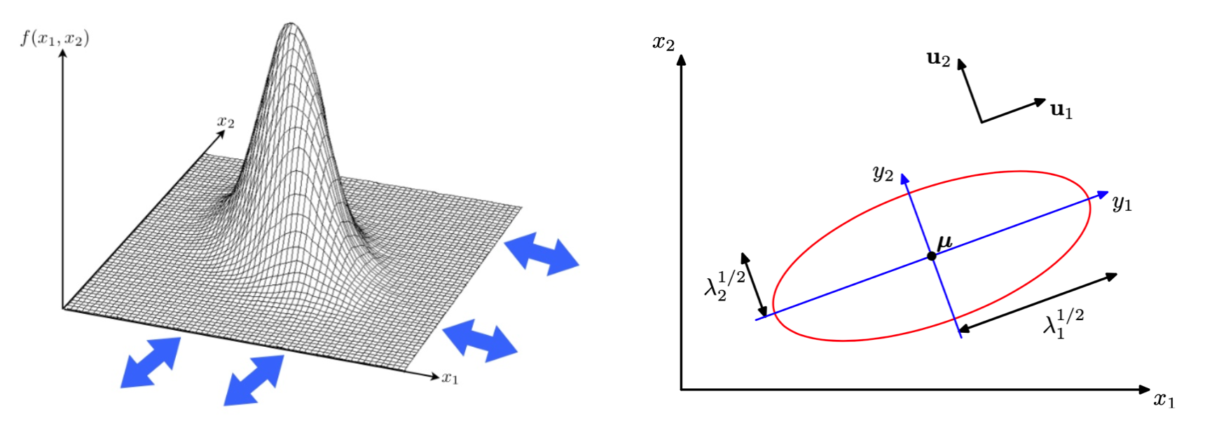
Fig. 20 Bivariate Gaussian density and ellipse
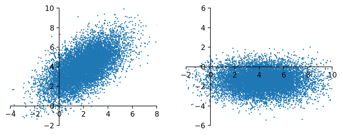
A numerical example to illustrate how \(\boldsymbol{\mu}, \boldsymbol{\Lambda} , \boldsymbol{U}\) jointly decide the distribution of \(\boldsymbol{x}\), and the effect of rotation transformation (rotation) \(\boldsymbol{U} ^{\top} \boldsymbol{x}\)
import numpy as np, pandas as pd, matplotlib.pyplot as plt
mu = [2,4]
Lam = np.diag([4,1])
U = np.asarray([[1,1], [1,-1]]/np.sqrt(2))
S = U @ Lam @ U.T
n = 10000
np.random.seed(1)
X = np.random.multivariate_normal(mean=mu, cov=S, size=n)
fig, ax = plt.subplots(1,2, figsize=(8,3), dpi=200)
ax[0].scatter(X[:,0], X[:,1], s=0.5)
ax[0].set_ylim(-2, 10)
ax[0].set_xlim(-4, 8)
ax[0].spines.left.set_position('zero')
ax[0].spines.bottom.set_position('zero')
ax[0].spines.right.set_color('none')
ax[0].spines.top.set_color('none')

# print(f'new center: {mu @ U.T}')
X2 = X @ U.T
ax[1].scatter(X2[:,0], X2[:,1], s=0.5)
ax[1].set_ylim(-6, 6)
ax[1].set_xlim(-2, 10)
ax[1].spines.left.set_position('zero')
ax[1].spines.bottom.set_position('zero')
ax[1].spines.right.set_color('none')
ax[1].spines.top.set_color('none')

plt.show()
Properties
Sometimes \(\boldsymbol{\varepsilon} \sim \mathcal{N} (\boldsymbol{0} , \boldsymbol{I} _p)\) is called white noise. If the off-diagonal entires are non-zero, we say there is ‘color’.
MGF: \(M_{\boldsymbol{x}}(\boldsymbol{t})=\exp \left(\boldsymbol{t}^{\top} \boldsymbol{\mu}+\frac{1}{2} \boldsymbol{t}^{\top} \boldsymbol{\Sigma} \boldsymbol{t}\right)\).
Sum: if \(\boldsymbol{x} \sim \mathcal{N} _p (\boldsymbol{\mu} _1, \boldsymbol{\Sigma} _1)\) and \(\boldsymbol{y} \sim \mathcal{N} _p (\boldsymbol{\mu} _2, \boldsymbol{\Sigma} _2)\) are independent, then \(\boldsymbol{x} + \boldsymbol{y} \sim \mathcal{N} _p (\boldsymbol{\mu} _1 + \boldsymbol{\mu} _2, \boldsymbol{\Sigma} _1 + \boldsymbol{\Sigma} _2)\).
What is the condition for a valid covariance matrix \(\boldsymbol{\Sigma}\)? Given a positive definite matrix \(\boldsymbol{\Sigma}\), then \(\boldsymbol{x} \sim \mathcal{N} _p (\boldsymbol{\mu} , \boldsymbol{\Sigma})\) iff there exists a non-singular matrix \(\boldsymbol{B}\) and \(\boldsymbol{z} \sim \mathcal{N} _p (\boldsymbol{0} , \boldsymbol{I})\) such that \(\boldsymbol{x} = \boldsymbol{\mu} + \boldsymbol{B} \boldsymbol{z}\). In this case \(\boldsymbol{\Sigma} = \boldsymbol{B} \boldsymbol{B} ^{\top}\).
Sub-vectors: if \(\boldsymbol{x} \in \mathcal{N} _{p + q} (\boldsymbol{\mu} , \boldsymbol{\Sigma})\), let \(\boldsymbol{x}_1\) be its first \(p\) components and \(\boldsymbol{x} _2\) be the rest \(q\) components, then
still normal: \(\boldsymbol{x}_{1} \sim \mathcal{N}_{p}\left(\boldsymbol{\mu}_{1}, \boldsymbol{\Sigma}_{11}\right), \boldsymbol{x}_{2} \sim \mathcal{N}_{q}\left(\boldsymbol{\mu}_{2}, \boldsymbol{\Sigma} _{22}\right)\)
\(\boldsymbol{x} _1\) and \(\boldsymbol{x} _2\) are independent iff \(\operatorname{Cov}\left( \boldsymbol{x} _1, \boldsymbol{x} _2 \right) = \boldsymbol{\Sigma} _{12} = \boldsymbol{0}_{p \times q}\) (hint for \(\Leftarrow\): use definition \(f_{12} = f_1 f_2\))
\((\boldsymbol{x} _1 - \boldsymbol{\Sigma} _{12} \boldsymbol{\Sigma} _{22} ^{-1} \boldsymbol{x} _2)\) is independent of \(\boldsymbol{x} _2\) and is distributed as \(\mathcal{N} _p (\boldsymbol{\mu} _1 - \boldsymbol{\Sigma} _{12} \boldsymbol{\Sigma} _{22} ^{-1} \boldsymbol{\mu} _2, \boldsymbol{\Sigma} _{11}- \boldsymbol{\Sigma} _{12} \boldsymbol{\Sigma} _{22} ^{-1} \boldsymbol{\Sigma} _{21})\).
conditional distribution is normal:
\[ \boldsymbol{x}_{1} \mid \boldsymbol{x}_{2} \sim N_{p}\left(\boldsymbol{\mu}_{1}+\boldsymbol{\Sigma}_{12} \boldsymbol{\Sigma}_{22}^{-1}\left(\boldsymbol{x}_{2}-\boldsymbol{\mu}_{2}\right), \boldsymbol{\Sigma}_{11}-\boldsymbol{\Sigma}_{12} \boldsymbol{\Sigma}_{22}^{-1} \boldsymbol{\Sigma}_{21}\right) \]Note the variance does not change with \(\boldsymbol{x} _2\). In particular,
for \(p=q=1\),
\[\begin{split} \begin{aligned} X_{1} \mid X_{2}=x_{2} \sim & N\left(\mu_{1}+\frac{\sigma_{12}}{\sigma_{22}}\left(x_{2}-\mu_{2}\right), \sigma_{11}-\frac{\sigma_{12}^{2}}{\sigma_{22}}\right) \\ &=N\left(\mu_{1}+\rho \frac{\sigma_{1}}{\sigma_{2}}\left(x_{2}-\mu_{2}\right), \sigma_{1}^{2}\left(1-\rho^{2}\right)\right) \end{aligned} \end{split}\]if \(p=1\), then \(x_1 = \mu_1 + \boldsymbol{\beta} ^{\top} (\boldsymbol{x} _2 - \boldsymbol{\mu} _2)\), i.e. a ‘regression’ model, where \(\boldsymbol{\beta} ^{\top} = \boldsymbol{\Sigma}_{12} \boldsymbol{\Sigma}_{22}^{-1}\). Let \(\boldsymbol{\Omega} = \boldsymbol{\Sigma} ^{-1}\), using block matrix inverse formula, it is easy to show that \(\beta_j = - \omega_{1j}/\omega_{11}\).
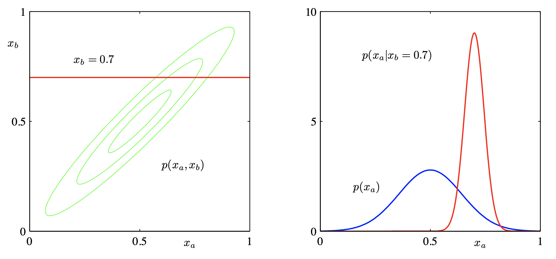
Fig. 21 Marginal Gaussian and conditional Gaussian are also Gaussians [Shi 2021]
Transformation: If \(\boldsymbol{x}\) is \(p\)-variate normal \(\mathcal{N} (\boldsymbol{\mu} , \boldsymbol{\Sigma})\), and \(\boldsymbol{y} = \boldsymbol{A} \boldsymbol{x} + \boldsymbol{c}\), where \(\boldsymbol{A}\) is a \(k \times p\) matrix and \(\boldsymbol{c}\) is a \(k\)-vector of constants, then \(\boldsymbol{y}\) is of \(k\)-variate normal, with mean \(\boldsymbol{A} \boldsymbol{\mu} + \boldsymbol{c}\) and variance \(\boldsymbol{A} \boldsymbol{\Sigma} \boldsymbol{A} ^{\top}\).
If \(k=1\), then \(\boldsymbol{y} = \boldsymbol{a} ^{\top} \boldsymbol{x} \sim \mathcal{N} ( \boldsymbol{a} ^{\top} \boldsymbol{\mu} , \boldsymbol{a} ^{\top} \boldsymbol{\Sigma} \boldsymbol{a})\)
if \(\boldsymbol{x}\) is standard normal \(\mathcal{N}(\boldsymbol{0}, \boldsymbol{I})\), then \(\boldsymbol{y} \sim \mathcal{N} (\boldsymbol{c} , \boldsymbol{A} \boldsymbol{A} ^{\top})\)
Independency after transformation: for any \(m\times p\) matrix \(\boldsymbol{A}\) and \(n\times p\) matrix \(\boldsymbol{B}\),
\(\boldsymbol{A} \boldsymbol{x} \perp \boldsymbol{B} \boldsymbol{x} \Leftrightarrow \boldsymbol{A} \boldsymbol{\Sigma} \boldsymbol{B} ^{\top} = \boldsymbol{0}\)
corollary: \(X_i \perp X_j \Leftrightarrow \sigma_{ij} =0\).
when \(\boldsymbol{A}\) is symmetric, \(\boldsymbol{x} ^{\top}\boldsymbol{A} \boldsymbol{x} \perp \boldsymbol{B} \boldsymbol{x} \Leftrightarrow \boldsymbol{B} \boldsymbol{\Sigma} \boldsymbol{A} = \boldsymbol{0}\)
when both \(\boldsymbol{A}, \boldsymbol{B}\) are symmetric, \(\boldsymbol{x} ^{\top}\boldsymbol{A} \boldsymbol{x} \perp \boldsymbol{x} ^{\top} \boldsymbol{B} \boldsymbol{x} \Leftrightarrow \boldsymbol{A} \boldsymbol{\Sigma} \boldsymbol{B} = \boldsymbol{0}\)
Since EVD \(\boldsymbol{\Sigma} = \boldsymbol{U} \boldsymbol{\Lambda} \boldsymbol{U} ^\top\), then \(\left\vert \boldsymbol{\Sigma} \right\vert = \left\vert \boldsymbol{U} \boldsymbol{\Lambda} \boldsymbol{U} ^\top \right\vert = \left\vert \boldsymbol{\Lambda} \right\vert\)
For every multivariate Gaussian \(\boldsymbol{x} \sim N(\boldsymbol{\mu} , \boldsymbol{\Sigma} )\) with \(\boldsymbol{\Sigma} = \boldsymbol{U} \boldsymbol{\Lambda} \boldsymbol{U} ^\top\), there exists a transformation \(\boldsymbol{x} ^\prime = \boldsymbol{U} ^\top \boldsymbol{x}, \boldsymbol{\mu} ^\prime = \boldsymbol{U} ^\top \boldsymbol{\mu}\) such that
\[ f(\boldsymbol{x} ; \boldsymbol{\mu}, \boldsymbol{\Sigma} ) = f(\boldsymbol{x} ^\prime ; \boldsymbol{\mu} ^\prime , \boldsymbol{\Lambda}) \]where
\[\begin{split}\begin{align} f(\boldsymbol{x} ^\prime ; \boldsymbol{\mu} ^\prime , \boldsymbol{\Lambda}) &= \frac{1}{(2 \pi)^{p / 2}|\boldsymbol{\Lambda}|^{1 / 2}} \exp \left(-\frac{1}{2}(\boldsymbol{x}^\prime -\boldsymbol{\mu} ^\prime )^{\top} \boldsymbol{\Lambda} ^{-1}( \boldsymbol{x} ^\prime -\boldsymbol{\mu} ^\prime )\right) \\ &= \frac{1}{(2 \pi)^{p / 2}\Pi_{i=1}^p \lambda_i} \exp \left(-\sum_{i=1}^p\frac{1}{2\sigma_{ii}}(x_i^\prime -\mu_i ^\prime )^2\right) \\ &= \prod_{i=1}^{p} \frac{1}{(2 \pi)^{1 / 2} \lambda_{i}} \exp \left(-\frac{1}{2 \lambda_{i}}\left(x_{i}^\prime -\mu_{i}^\prime \right)^{2}\right) \end{align}\end{split}\]which is a product of PDFs of univariate Gaussians, i.e. dependency is dropped. Geometrically, \(\boldsymbol{U}\) rotate the axes of the distribution but keep the function value intact.
Quadratic form: if \(\boldsymbol{x} \sim \mathcal{N} _p (\boldsymbol{\mu} , \boldsymbol{\Sigma})\) and \(\boldsymbol{\Sigma}\) is p.d., then \((\boldsymbol{x} - \boldsymbol{\mu} ) ^{\top} \boldsymbol{\Sigma} ^{-1} (\boldsymbol{x} - \boldsymbol{\mu} ) \sim \chi ^2 _p\).
For standard Gaussian \(\boldsymbol{z} \sim \mathcal{N} _p (\boldsymbol{0} , \boldsymbol{I})\): $\(\boldsymbol{z} ^{\top} \boldsymbol{z} = \sum_{j=1}^p Z_i^2 \sim \chi ^2 _p\)$
In sample data, as \(n\) is large, \(n(\bar{\boldsymbol{x}}-\boldsymbol{\mu})^{\prime} \boldsymbol{S}^{-1}(\bar{\boldsymbol{x}}-\boldsymbol{\mu}) \sim \chi_{p}^{2}\)
Related to unit surface: if \(\boldsymbol{x}\) follow spherical Gaussian \(\mathcal{N}_p (\boldsymbol{0} , \sigma^2 \boldsymbol{I} _p)\), let the norm be \(R = \left\| \boldsymbol{x}\right\|\), then its density is
\[ f_p(r) = \frac{S_p}{ (2 \pi \sigma^2)^{p / 2}} r^{p -1} \exp \left( -\frac{r^2}{2 \sigma^2 } \right), \quad r \ge 0 \]where \(S_p=\frac{2 \pi^{p / 2}}{\Gamma(p / 2)}\) is the surface area of the unit sphere in \(p\)-dimensions.
When \(r= \sqrt{\sigma^2 (p-1)}\), \(f_p(r)\) achieves its maximum. That is, it characterizes the unit spherical shell that has the ‘most’ points on it among all unit spherical shells in \(\mathbb{R} ^p\).
if \(\sigma^2\) is fixed, then the optimal radius scales sub-linearly in \(d\), i.e. \(r^* = \mathcal{O}(\sqrt{p})\)
if we set \(\sigma^2 = 1/d\), then \(r = \sqrt{(p-1)/p} \approx 1\). See below.
In high-dimensional case, as \(p \rightarrow \infty\),
independent Gaussian points with variance \(\frac{1}{p}\) concentrate on the surface of sphere \(S^{p-1}\), i.e.
\[\mathcal{N} _p (\boldsymbol{0} , p ^{-1} \boldsymbol{I} _p) \approx \operatorname{Unif} (S^{p-1})\]for \(\boldsymbol{x} , \boldsymbol{y} \sim \mathcal{N} _p(\boldsymbol{0} , \frac{1}{p} \boldsymbol{I} _p)\), we have
\(\mathbb{E} [\boldsymbol{x} ^{\top} \boldsymbol{x} ] = \sum_{i=1}^p \mathbb{E} [X_j^2] = \sum_{j=1}^p \frac{1}{p} = 1\)
\(\mathbb{E} [\boldsymbol{x} ^{\top} \boldsymbol{y} ] = \sum_{j=1}^p \mathbb{E} [X_j Y_j] = \sum_{j=1}^p \mathbb{E} [X_j] \mathbb{E} [Y_j] = 0\).
\(\mathbb{E} [\left\| \boldsymbol{a} ^{\top} \boldsymbol{x} \right\| ^2 ] = \sum_{j=1}^p a_j ^2 \mathbb{E} [X_j^2] + \sum_{j\ne k}^p a_j a_k \mathbb{E} [X_j X_k] = \sum_{j=1}^p \frac{a_j^2}{p} = \frac{1}{p} \left\| \boldsymbol{a} \right\|^2\)
\(\left\| \boldsymbol{x} \right\| \rightarrow 1\)
\(\boldsymbol{x} ^{\top} \boldsymbol{y} \rightarrow 0\)
\(\boldsymbol{a} ^{\top} \boldsymbol{x} \rightarrow 0\) for \(\left\| \boldsymbol{a} \right\| =1\).
Estimation
MLE
The MLE of \(\boldsymbol{\mu}\) and \(\boldsymbol{\Sigma}\) are respectively
Note that \(\hat{\boldsymbol{\mu}}\) is unbiased but \(\hat{\boldsymbol{\Sigma} }\) is unbiased. However, \(\boldsymbol{S}\) is unbiased for \(\boldsymbol{\Sigma}\).
Wishart Distribution
Recall that for univariate i.i.d. standard Gaussians we have \(\sum_{i=1}^k Z_i^2 \sim \sigma^2 \chi ^2 _n\). The multivariate extension of this chi-squared distribution is Wishart distribution.
- Definition (Wishart distribution)
Suppose \(\boldsymbol{x}_1, \ldots, \boldsymbol{x} _k\) and independent \(\mathcal{N} _p (\boldsymbol{\mu} _i, \boldsymbol{\Sigma})\). Define a symmetric \(p \times p\) matrix \(\boldsymbol{V}\) as
\[ \boldsymbol{V} = \sum_{i=1}^k \boldsymbol{x} _i \boldsymbol{x}_i ^{\top} = \boldsymbol{X} ^{\top} \boldsymbol{X} \]Then \(\boldsymbol{V}\) is said to follow a Wishart distribution \(W_p(k, \boldsymbol{\Sigma} , \boldsymbol{\Psi})\), where
\(n\) is the degree of freedom
\(\boldsymbol{\Sigma}\) is called the scaling matrix
\(\boldsymbol{\Psi} = \sum_{i=1}^k \boldsymbol{\mu} _i \boldsymbol{\mu} _i ^{\top}\) is the \(p \times p\) symmetric non-centrality matrix
If \(\boldsymbol{\Psi} = \boldsymbol{0}\), it is called the central Wishart distribution, denoted by \(W_p(k, \boldsymbol{\Sigma})\)
When \(p=1\) and \(\boldsymbol{\Sigma} = \sigma^2\), it reduces to a non-central chi-sqaured distribution \(\sigma^2 \chi ^2 (k, \sum_{i=1}^k \boldsymbol{\mu} _i^2)\).
- Properties
sum of independent: if \(\boldsymbol{V} _1 \sim W_p(k, \boldsymbol{\Sigma} , \boldsymbol{\Psi} _1)\) and \(\boldsymbol{V} _2 \sim W_p(k, \boldsymbol{\Sigma} , \boldsymbol{\Psi} _2)\) are independent Wisharts, then \(\boldsymbol{V} _1 + \boldsymbol{V} _2 \sim W_p (k_1 + k_2, \boldsymbol{\Sigma} , \boldsymbol{\Psi} _1 + \boldsymbol{\Psi} _2)\).
transformation: if \(\boldsymbol{V} \sim W_p (k, \boldsymbol{\Sigma} , \boldsymbol{\Psi})\), then
for any constant \(q \times p\) matrix \(\boldsymbol{A}\), \(\boldsymbol{A} \boldsymbol{V} \boldsymbol{A} ^{\top} \sim W_q (k, \boldsymbol{A} \boldsymbol{\Sigma} \boldsymbol{A} ^{\top} , \boldsymbol{A} \boldsymbol{\Psi} \boldsymbol{A} ^{\top})\).
for any constant \(\boldsymbol{a}\), \(\boldsymbol{a}^{\top} \boldsymbol{V} \boldsymbol{a} / \boldsymbol{a}^{\top} \boldsymbol{\Sigma} \boldsymbol{a} \sim \chi^{2}\left(k, \boldsymbol{a}^{\top} \boldsymbol{\Psi} \boldsymbol{a}\right)\). In particular, \(v_{ii}/\sigma_{ii} \sim \chi ^2 (k, \Phi_{ii})\).
for any random vector \(\boldsymbol{y}\) independent of \(\boldsymbol{V} \sim W_p(k, \boldsymbol{\Sigma})\),
\(\boldsymbol{y}^{\top} \boldsymbol{V} \boldsymbol{y} / \boldsymbol{y}^{\top} \boldsymbol{\Sigma} \boldsymbol{y} \sim \chi^{2}(k)\) and is independent of \(\boldsymbol{y}\).
\(\boldsymbol{y}^{\top} \boldsymbol{\Sigma}^{-1} \boldsymbol{y} / \boldsymbol{y}^{\top} \boldsymbol{V}^{-1} \boldsymbol{y} \sim \chi^{2}(k-p+1)\) if \(k > p\), and is independent of \(\boldsymbol{y}\).
for random \(k \times p\) matrix \(\boldsymbol{X}\),
for a symmetric \(\boldsymbol{A}: \boldsymbol{X}^{\top} \boldsymbol{A} \boldsymbol{X} \sim W_{p}(r, \boldsymbol{\Sigma}, \boldsymbol{\Psi}) \Leftrightarrow \boldsymbol{A} ^2 = \boldsymbol{A}\) (idempotent), in which case \(r=\operatorname{rank}(\boldsymbol{A})=\operatorname{tr}(\boldsymbol{A})\) and \(\boldsymbol{\Psi}=\boldsymbol{M}^{\top} \boldsymbol{A} \boldsymbol{M}\)
for symmetric idempotent \(\boldsymbol{A}, \boldsymbol{B}\), we have \(\boldsymbol{X} ^{\top} \boldsymbol{A} \boldsymbol{X} \perp \boldsymbol{X} ^{\top} \boldsymbol{B} \boldsymbol{X} \Leftrightarrow \boldsymbol{A} \boldsymbol{B} = \boldsymbol{0}\).
for symmetric idempotent \(\boldsymbol{A}\), we have \(\boldsymbol{X} ^{\top} \boldsymbol{A} \boldsymbol{X} \perp \boldsymbol{X} ^{\top} \boldsymbol{B} \Leftrightarrow \boldsymbol{A} \boldsymbol{B} = \boldsymbol{0}\).
Gaussian MLE
\(\bar{\boldsymbol{x}} \sim \mathcal{N} _p (\boldsymbol{\mu} , \frac{1}{n} \boldsymbol{\Sigma} )\)
\((n-1) \boldsymbol{S} = \boldsymbol{W} \sim W_p(n-1, \boldsymbol{\Sigma})\), extension of \(\sum_{i=1}^n (x_i - \bar{x})^2 \sim \sigma^2\chi ^2 _{n-1}\)
\(\bar{\boldsymbol{x} } \perp \boldsymbol{S}\)
In the Cholesky decomposition \(\boldsymbol{V} = \boldsymbol{T} \boldsymbol{T} ^{\top}\) of \(\boldsymbol{V} \sim W_p (k, \boldsymbol{\Sigma})\), where \(\boldsymbol{T}\) is lower triangular,
off-diagonal \(t_{ij} \sim \mathcal{N} (0,1)\) for \(i >j\)
diagonal \(t_{ii} \sim \chi ^2 _{k-i+1}\)
all non-zero elements are mutually independent
If \(\boldsymbol{x}_i \sim \mathcal{N} (\boldsymbol{0} , \boldsymbol{I} _p)\), then the eigenvalues of a \(\frac{1}{n} \boldsymbol{X} ^{\top} \boldsymbol{X}\), as \(p, n \rightarrow \infty\), follows Marchenko–Pastur distribution.
Pros and Cons
Pros
Related to CLM
Evaluation is convenient
Can be convert to product of univariate Gaussians in some rotated space
Mixtures of Gaussian are sufficient to approximate a wide range of distributions
Arbitrary linear combinations of jointly Gaussian variables are also Gaussian
Marginals and conditionals of multivariate Gaussians are also Gaussian
Sums of many i.i.d. random variables converge to Gaussian variables (Central Limit Theorem)
Log of Gaussian looks like a weighted Euclidean distance, related to squared loss
\[ -\ln \sqrt{(2 \pi \sigma)}-\frac{(x-\mu)^{2}}{\left(2 \sigma^{2}\right)} \]
Cons
\(\boldsymbol{\Sigma}\) is hard and expensive to estimate in high dimensions
sol: assume special structure: diagonal, spherical
Normality Check
For most univariate/multivariate analyses, it is important that the data indeed follow the normal distribution, at least approximately if not exactly.
Qualitative Ways
QQ-plots (quantile-quantile plot)
Sample quantiles are plotted against the expected sample quantiles of a standard normal distribution
If the points lie on a straight line, then it indicates univariate normality. In addition to measure this linearity by eye, we can also use correlation coefficient to quantify it.
non-linearity may indicate a need to transform the variable.
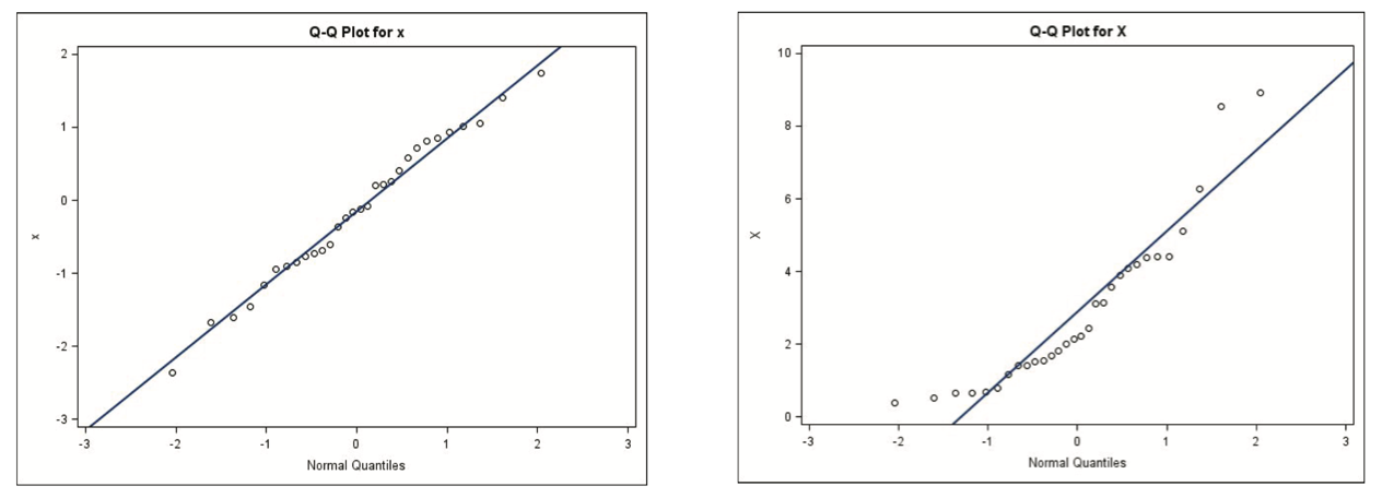
Fig. 22 QQ-plots for Gaussian (left) and non-Gaussian (right)
P-P plot (probability against probability plot) that plots the sample CDF against the theoretical CDF.
Among all continuous random variable with mean \(0\), variance \(\sigma^2\), normal random variable has the largest differential entropy with value \(\operatorname{H}(\mathcal{N}(0, \sigma^2)) = \ln(\sigma \sqrt{2 \pi e})\). Hence, the distance of an entropy from the normal entropy (termed neg-entropy), can be used to develop measures of non-Gaussianity, or non-normality.
Rigorous Tests
Shapiro–Wilk \(W\) test
test statistic: a modified version of the squared sample correlation between the sample quantiles and the expected quantiles.
Kolmogorov–Smirnov test
Require: large sample, at least 100s
Test statistic: maximum difference between the empirical CDF and the normal CDF.
Jarque–Bera test
Test for zero skewness, zero excess kurtosis.
Normal distribution has kurtosis \(\frac{\mu_{4}}{\mu_{2}^{2}}=3\) and excess kurtosis \(\frac{\mu_{4}}{\mu_{2}^{2}}-3 = 0\). Large magnitude of excess kurtosis indicates deviation from normal distribution.
Multivariate Cases
Check whether the squared generalized distance as defined below follows a chi-squared distribution by a Q-Q plot (necessary and sufficient conditions for very large sample size))
\[ d_{i}^{2}=\left(\boldsymbol{x}_{i}-\overline{\boldsymbol{x}}\right)^{\prime} \boldsymbol{S}^{-1}\left(\boldsymbol{x}_{i}-\overline{\boldsymbol{x}}\right) \]Again, correlation coefficient can be used to quantity the linearity of the points.
Check each Principal Component (PC) for univariate normality (necessary condition; and if the sample size n is large enough, a sufficient condition)
Transformation to Near Normality
To achieve the multinormality of the data, univariate transformation is applied to each variable individually. After then, the multinormality of transformed variables is checked again (Notice that each of the \(X_p\) variables after transformation is normally distributed does not imply that they jointly follow a multivariate normal distribution).
Assume \(x > 0\).
common method \(\log x\)
based on theory:
Poisson count: \(\sqrt{x}\)
Binomial proportion: \(\sin ^{-1} \sqrt{x}\)
Box-Cox transformation
\[\begin{split} x_{i}^{[\lambda]}=\left\{\begin{array}{lll} \frac{x_{i}^{\lambda}-1}{\lambda} & \text { for } \lambda \neq 0 & , i=1, \ldots, n \\ \log x_{i} & \text { for } \lambda=0 & , i=1, \ldots, n \end{array}\right. \end{split}\]where \(\lambda\) is unknown. It can be chosen by priori information of \(\lambda\), or search among some values \(3,2,1,\frac{1}{2}, \frac{1}{3}, 0\) and their negatives.
Cons:
Box-Cox transformation cannot guarantee that the transformed variable is close to the normal distribution.
Choice of \(\lambda\) depends on scale of \(x_i\). Sol: power transform
Power transform, where \(G M(x)=\left(x_{1} x_{2} \cdots x_{n}\right)^{1 / n}\) is the geometric mean of observations.
\[\begin{split} x_{i}^{[\lambda]}=\left\{\begin{array}{ll} \frac{x_{i}^{\lambda}-1}{\lambda[G M(x)]^{\lambda-1}}, & \text { if } \lambda \neq 0 \quad, i=1, \ldots, n \\ G M(x) \log x_{i}, & \text { if } \lambda=0 \quad, i=1, \ldots, n \end{array}\right. \end{split}\]The optimal \(\lambda\) minimizes sample variance after transformation.