Linear Models - Estimation¶

From this section we introduce linear models from a statistics’ perspective. There are three sections in total.

The first section covers the model fundamentals, including assumptions, estimation, interpretation and some exercise.
The next section introduce statistical inference for linear models, such as distribution of the estimated coefficients, $t$-test, $F$-test, etc. Usually machine learning community focuses more on prediction, less on inference. But inference does matters. It analyzes how important each variable is in the model from a rigorous approach.
The third section introduce some issues in linear models, e.g. omitted variables bias, multicollinearity, heteroskedasticity, and some alternative models, e.g. Lasso, ridge regression, etc.

Statistics’ perspective vs social science’s perspective

The introduction from econometrics’ perspective or social science’s perspective may be different. In short, the statistics’ perspective focuses on general multivariate cases and heavily rely on linear algebra for derivation, while the econometrics’ or the social science’s perspective prefers to introduce models in univariate cases by basic arithmetics (whose form can be complicated without linear algebra notations) and extend the intuitions and conclusions into multivariate cases.

Personally, I involved in four courses that introduced linear models, i.e. at undergrad/grad level offered by stat/social science department. The style of the two courses offered by the stat departments were quite alike while the graduate level one covered more topics. In both undergrad/grad level courses offered by the social science departments, sometimes I got confused by the course materials that were contradictory to my statistics training , but the instructors had no clear response or even no response at all…

In sum, to fully understand the most fundamental and widely used statistical model, I highly suggest to take a linear algebra course first and take the regression course offered by math/stat department.

Objective¶

Linear models aim to model the relationship between a scalar response and one or more explanatory variables in a linear format:

\[Y_i = \beta_0 + \beta_1 x_{i,1} + \ldots + \beta_{p-1} x_{i,p-1} + \varepsilon_i \]

for observations $i=1, 2, \ldots, n$.

In matrix form,

\[ \boldsymbol{y} = \boldsymbol{X} \boldsymbol{\beta} + \boldsymbol{\varepsilon}. \]

where

$\boldsymbol{X}_{n\times p}$ is called the design matrix. The first column is usually set to be $\boldsymbol{1}$, i.e., intercept. The remaining $p-1$ columns are designed values $x_{ij}$ where $i = 1, 2, \ldots, n$ and $j=1, \ldots, p-1$. These $p-1$ columns are called explanatory/independent variables, or covariates.
$\boldsymbol{y}_{n \times 1}$ is a vector of response/dependent variables $Y_1, Y_2, \ldots, Y_n$.
$\boldsymbol{\beta}_{p \times 1}$ is a vector of coefficients to be estimated.
$\boldsymbol{\varepsilon}_{n \times 1}$ is a vector of unobserved random errors, which includes everything that we have not measured and included in the model.

When $p=2$, we have

\[ Y_i = \beta_0 + \beta_1 x_i + \varepsilon_i \]

which is called simple linear regression.

When $p>2$, it is called multiple linear regression. For instance, when $p=3$

\[ Y_i = \beta_0 + \beta_1 x_1 + \beta_2 x_2 + \varepsilon_i \]

When there are multiple dependent variables, we call it multivariate regression, which will be introduced in another section.

When $p=1$,

if we include intercept, then the regression model $y_i = \beta_0$ means that we use a single constant to predict $y_i$. The estimator, $\hat{\beta}_0$, by ordinary least square, should be the sample mean $\hat{y}$.
if we do not include intercept, then the regression model $y_i = \beta x_i$ means that we expect that $y$ is proportional to $x$.

Fixed or random $\boldsymbol{X}$?

In natural science, researchers design $n\times p$ values in the design matrix $\boldsymbol{X}$ and run experiments to obtain the response $y_i$. We call this kind of data experimental data. In this sense, the explanatory variables $x_{ij}$’s are designed before the experiment, so they are also constants. The coefficients $\beta_j$’s are unknown constants. The error term $\varepsilon_i$ is random. The response variable $Y_i$ on the left hand side is random due to the randomness in the error term $\varepsilon_i$.

In social science, most of data is observational data. That is, researchers obtain the values of many variables at the same time, and choose one of interest to be the response variable $y_i$ and some others to be the explanatory variables $\boldsymbol{x}_i$. In this case, $\boldsymbol{X}$ is viewed as a data set, and we can talk about descriptive statistics, such as variance of each explanatory variable, or covariance between pair of explanatory variables. This is valid since we often view the columns of a data set as random variables.

However, the inference methods of the coefficients $\boldsymbol{\beta}$ are developed based on the natural science setting, i.e., the values of explanatory variables are pre-designed constants. Many social science courses frequently use descriptive statistics of the explanatory variables which assumes they are random, and apply inference methods which assumes they are constant. This is quite confusing for beginners to linear models.

To be clear, we stick to the natural science setting and make the second assumption below. We use subscript $i$ in every $y_i, x_i, \varepsilon_i$ instead of $y, x, \varepsilon$ which gives a sense that $x$ is random. And we use descriptive statistics for the explanatory variables only when necessary.

Assumptions¶

Basic assumptions

$\operatorname{E}\left( y_i \right) = \boldsymbol{x}_i ^\top \boldsymbol{\beta}$ is linear in covariates $X_j$.
The values of explanatory variables $\boldsymbol{x}_i$ are known and fixed. Randomness only comes from $\varepsilon_i$.
No $X_j$ is constant for all observations. No exact linear relationships among the explanatory variables (aka no perfect multicollinearity, or the design matrix $\boldsymbol{X}$ is of full rank).
The error terms are uncorrelated $\operatorname{Cov}\left( \varepsilon_i, \varepsilon_j \right)= 0$, with common mean $\operatorname{E}\left( \varepsilon_i \right) = 0$ and variance $\operatorname{Var}\left( \varepsilon_i \right) = \sigma^2$ (homoskedasticity).

As a result, $\operatorname{E}\left( \boldsymbol{y} \mid \boldsymbol{X} \right) = \boldsymbol{X} \boldsymbol{\beta}$, or $\operatorname{E}\left( y_i \mid x_i \right) = \beta_0 + \beta_1 x_i$ when $p=2$, which can be illustrated by the plots below.

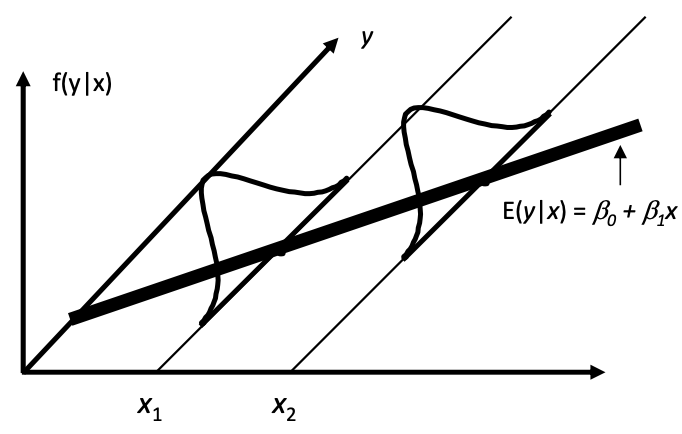
Fig. 58 Distributions of $y$ given $x$ [Meyer 2021]¶

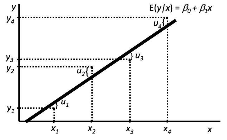
Fig. 59 Observations of $y$ given $x$ [Meyer 2021]¶

To predict $\hat{y}_i$, we just use $\hat{y}_i = \boldsymbol{x}_i ^\top \hat{\boldsymbol{\beta}}$ .
The error terms are independent and follow Gaussian distribution $\varepsilon_i \overset{\text{iid}}{\sim}N(0, \sigma^2)$, or $\boldsymbol{\varepsilon} \sim N_n (\boldsymbol{0} , \sigma^2 \boldsymbol{I} _n)$.

As a result, we have $Y_i \sim N(\boldsymbol{x}_i ^\top \boldsymbol{\beta} , \sigma^2 )$ or $\boldsymbol{y} \sim N_n(\boldsymbol{X} \boldsymbol{\beta} , \sigma^2 \boldsymbol{I} _n)$

These assumptions are used for different objectives. The first 3 assumptions are the base, and in additiona to them,

derivation of $\hat{\boldsymbol{\beta}}$ by least squares uses no more assumptions.
derivation of $\hat{\boldsymbol{\beta}}$ by maximal likelihood uses assumptions 4 and 5.
derivation of $\operatorname{E}\left( \hat{\boldsymbol{\beta}} \right)$ uses $\operatorname{E}\left( \varepsilon_i \right) = 0$ in 4.
derivation of $\operatorname{Var}\left( \hat{\boldsymbol{\beta}} \right)$ uses 1, 2, $\operatorname{Cov}\left( \varepsilon_i, \varepsilon_j \right) = 0$ and $\operatorname{Var}\left( \epsilon_i \right) = \sigma^2$ in 4.
proof of Gaussian-Markov Theorem (BLUE) uses 4.
derivation of the distribution of $\hat{\boldsymbol{\beta} }$ uses 4 and 5.

Zero conditional mean assumption

In some social science or econometrics courses, they follow the “Gauss-Markov assumptions” that are roughly the same to the assumptions, but in different formats. One of them is zero conditional mean assumption.

In general, it says

\[ \operatorname{E}\left( \varepsilon \mid x_1, x_2, \ldots, x_p\right) = 0 \]

For $p=2$, it is

\[\operatorname{E}\left( \varepsilon \mid x \right) = 0\]

which (in their setting) implies

\[\begin{split}\begin{align} \operatorname{E}\left( \varepsilon \right) &= \operatorname{E}\left( \operatorname{E}\left( \varepsilon \mid x \right) \right)\\ &= 0\\ \operatorname{Cov}\left( \varepsilon, x \right) &= \operatorname{E}\left( \varepsilon x \right) - \operatorname{E}\left( \varepsilon \right)\operatorname{E}\left( x \right)\\ &= \operatorname{E}\left( \operatorname{E}\left( \varepsilon x \mid x \right) \right)- 0 \times \operatorname{E}\left( x \right)\\ &= \operatorname{E}\left( x \operatorname{E}\left( \varepsilon \mid x \right) \right) \\ &= 0 \end{align}\end{split}\]

Then they these two corollaries are used for estimation.

As discussed above, in their setting $x$ is random (at this stage), so they use notations such as $\operatorname{E}\left( \varepsilon \mid x \right)$ and $\operatorname{Cov}\left( x, \varepsilon \right)$. It also seems that they view $\varepsilon$ as an “overall” measure of random error, instead of $\varepsilon_i$ for specific $i$ in the natural science setting. But they can mean so by using the conditional notation $\operatorname{E}\left( \varepsilon \mid x \right)$.

Estimation¶

We introduce various methods to estimate the parameters $\boldsymbol{\beta}$ and $\sigma^2$.

Ordinary Least Squares¶

The most common way is to estimate the parameter $\hat{\boldsymbol{\beta}}$ by minimizing the sum of squared errors $\sum_i(y_i-\hat{y}_i)^2$.

\[\begin{split}\begin{align} \hat{\boldsymbol{\beta}} &= \underset{\boldsymbol{\beta} }{\mathrm{argmin}} \, \left\Vert \boldsymbol{y} - \hat{\boldsymbol{y}} \right\Vert ^2 \\ &= \underset{\boldsymbol{\beta} }{\mathrm{argmin}} \, \left\Vert \boldsymbol{y} - \boldsymbol{X} \boldsymbol{\beta} \right\Vert ^2 \\ \end{align}\end{split}\]

The gradient w.r.t. $\boldsymbol{\beta}$ is

\[\begin{split}\begin{align} \nabla_{\boldsymbol{\beta}} &= -2 \boldsymbol{X} ^\top (\boldsymbol{y} - \boldsymbol{X} \boldsymbol{\beta} ) \\ &\overset{\text{set}}{=} \boldsymbol{0} \end{align}\end{split}\]

Hence, we have

\[ \boldsymbol{X} ^\top \boldsymbol{X} \boldsymbol{\beta} = \boldsymbol{X} ^\top \boldsymbol{y} \]

This linear system is called the normal equation.

The closed form solution is

\[\hat{\boldsymbol{\beta}} = \left( \boldsymbol{X} ^\top \boldsymbol{X} \right)^{-1}\boldsymbol{X} ^\top \boldsymbol{y} \]

Note that $\hat{\boldsymbol{\beta}}=(\boldsymbol{X} ^\top \boldsymbol{X} ) ^{-1} \boldsymbol{X}^\top \boldsymbol{y}$ is a random variable, since it is a linear combination of the random vector $\boldsymbol{y}$. This means that, keeping $\boldsymbol{X}$ fixed, repeat the experiment, we will probably get different response values $\boldsymbol{y}$, and hence different $\hat{\boldsymbol{\beta}}$. As a result, there is a sampling distribution of $\hat{\boldsymbol{\beta}}$, and we can find its mean, variance, and conduct hypothesis testing.

View least squares as projection

Substitute the solve $\hat{\boldsymbol{\beta}}$ into the prediction $\hat{\boldsymbol{y}}$ we have

\[ \hat{\boldsymbol{y}} = \boldsymbol{X} \hat{\boldsymbol{\beta}} = \underbrace {\boldsymbol{X} (\boldsymbol{X} ^\top \boldsymbol{X} ) ^{-1} \boldsymbol{X} ^\top}_{\boldsymbol{H}} \boldsymbol{y} \]

Here $\boldsymbol{H}$ is a projection matrix onto the column space (image) of $\boldsymbol{X}$. Recall that a projection matrix onto the column span of a matrix $\boldsymbol{X}$ has the form $\boldsymbol{P} _{\operatorname{col}(\boldsymbol{X} )} = \boldsymbol{X} \boldsymbol{X} ^\dagger$ where $\boldsymbol{X} ^\dagger = (\boldsymbol{X} ^\top \boldsymbol{X} ) ^{-1} \boldsymbol{X} ^\top$ is the pseudo inverse of $\boldsymbol{X}$.

Essentially, we are trying to find a vector $\hat{\boldsymbol{y}}$ in the column space of the data matrix $\boldsymbol{X}$ that is as close to $\boldsymbol{y}$ as possible, and the closest one is just the projection of $\boldsymbol{y}$ onto $\operatorname{col}(\boldsymbol{X})$, which is $\boldsymbol{H}\boldsymbol{y}$. The distance is measured by the norm $\left\| \boldsymbol{y} - \hat{\boldsymbol{y}} \right\|$, which is the squared root of sum of squared errors. Note that $\boldsymbol{y} - \hat{\boldsymbol{y}} = (\boldsymbol{I} - \boldsymbol{H} ) \boldsymbol{y} \in \operatorname{col}(\boldsymbol{X}) ^ \bot$ since $\boldsymbol{I} - \boldsymbol{H} = \boldsymbol{I} - \boldsymbol{P}_{\operatorname{col}(\boldsymbol{X}) } = \boldsymbol{P}_{\operatorname{col}(\boldsymbol{X}) ^ \bot}$ is the projection matrix onto the orthogonal complement $\operatorname{col}(\boldsymbol{X}) ^ \bot$.

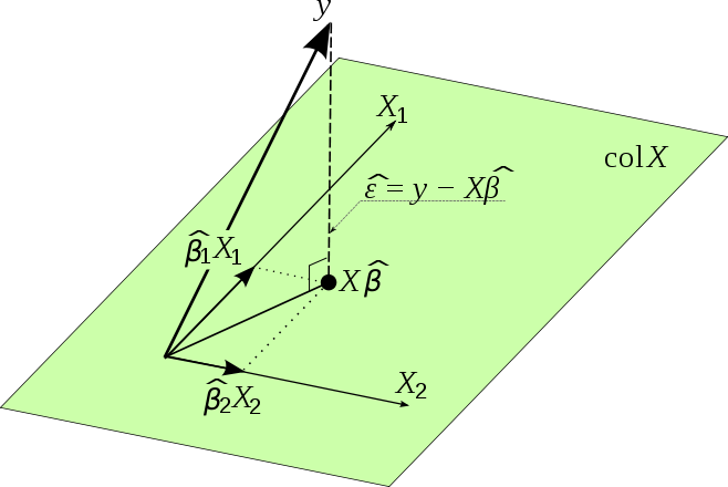
Fig. 60 Least squares as a projection [Gold 2017]¶

Solving the linear system by software

Computing software use specific functions to solve the normal equation $\boldsymbol{X} ^\top \boldsymbol{X} \boldsymbol{\beta} = \boldsymbol{X} ^\top \boldsymbol{y}$ for $\boldsymbol{\beta}$, instead of using the inverse $(\boldsymbol{X} ^\top \boldsymbol{X}) ^{-1}$ directly which can be slow and numerically unstable. For instance, one can use QR factorization of $X$,

\[\begin{split} \boldsymbol{X} = \boldsymbol{Q} \left[\begin{array}{l} \boldsymbol{R}_{p \times p} \\ \boldsymbol{0}_{(n-p) \times p} \end{array}\right] \end{split}\]

Hence,

\[\begin{split} \begin{aligned} \| \boldsymbol{y} - \boldsymbol{X} \boldsymbol{\beta} \|^{2} &=\left\|\boldsymbol{Q} ^{\top} \boldsymbol{y} - \boldsymbol{Q} ^\top \boldsymbol{X} \boldsymbol{\beta} \right\|^{2} \\ &=\left\|\left(\begin{array}{c} \boldsymbol{f} \\ \boldsymbol{r} \end{array}\right)-\left(\begin{array}{c} \boldsymbol{R} \boldsymbol{\beta} \\ \boldsymbol{0} \end{array}\right)\right\|^{2} \\ &=\|\boldsymbol{f} - \boldsymbol{R} \boldsymbol{\beta} \|^{2}+\|\boldsymbol{r} \|^{2} \end{aligned} \end{split}\]

Finally

\[ \boldsymbol{\beta} = \boldsymbol{R} ^{-1} \boldsymbol{f} \]

An unbiased estimator of the error variance $\sigma^2 = \operatorname{Var}\left( \varepsilon \right)$ is (to be discussed [later])

\[ \hat{\sigma}^2 = \frac{\left\Vert \boldsymbol{y} - \boldsymbol{X} \hat{\boldsymbol{\beta}} \right\Vert ^2}{n-p} \]

When $p=2$, we have

\[\hat{\beta}_0, \hat{\beta}_1 = \underset{\beta_0, \beta_1 }{\mathrm{argmin}} \, \sum_i \left( y_i - \beta_0 - \beta_1 x_i \right)^2\]

Differentiation w.r.t. $\beta_1$ gives

\[ - 2\sum_i (y_i - \beta_0 - \beta_1 x_i) x_i = 0 \]

Differentiation w.r.t. $\beta_0$ gives

\[ - 2\sum_i (y_i - \beta_0 - \beta_1 x_i) = 0 \]

Solve the system of the equations, we have

\[\begin{split}\begin{align} \hat{\beta}_{1} &=\frac{\sum_{i=1}^{n}\left(x_{i}-\bar{x}\right)\left(y_{i}-\bar{y}\right)}{\sum_{i=1}^{n}\left(x_{i}-\bar{x}\right)^{2}} \\ \hat{\beta}_{0} &=\bar{y}-\hat{\beta}_{1} \bar{x} \end{align}\end{split}\]

The expression for $\hat{\beta}_0$ implies that the fitted line cross the sample mean point $(\bar{x}, \bar{y})$.

Moreover,

\[ \hat{\sigma}^2 = \frac{1}{n-2} \sum_i \hat\varepsilon_i^2 \]

where $\hat\varepsilon_i = y_i - \hat{\beta}_0 - \hat{\beta}_1 x_i$.

Minimizing mean squared error

The objective function, sum of squared errors,

\[ \left\Vert \boldsymbol{y} - \boldsymbol{X} \boldsymbol{\beta} \right\Vert ^2 = \sum_i \left( y_i - \boldsymbol{x}_i ^\top \boldsymbol{\beta} \right)^2 \]

can be replaced by mean squared error,

\[ \frac{1}{n} \sum_i \left( y_i - \boldsymbol{x}_i ^\top \boldsymbol{\beta} \right)^2 \]

and the results are the same.

By Assumptions¶

In some social science courses, the estimation is done by using the assumptions

$\operatorname{E}\left( \varepsilon \right) = 0$
$\operatorname{E}\left( \varepsilon \mid X \right) = 0$

The first one gives

\[ \frac{1}{n} \sum_{i=1}^{n}\left(y_{i}-\hat{\beta}_{0}-\hat{\beta}_{1} x_{i}\right)=0 \]

The second one gives

\[\begin{split}\begin{align} \operatorname{Cov}\left( X, \varepsilon \right) &= \operatorname{E}\left( X \varepsilon \right) - \operatorname{E}\left( X \right) \operatorname{E}\left( \varepsilon \right) \\ &= \operatorname{E}\left[ \operatorname{E}\left( X \varepsilon \mid X \right) \right] - \operatorname{E}\left( X \right)\operatorname{E}\left[ \operatorname{E}\left( \varepsilon \mid X\right) \right]\\ &= \operatorname{E}\left[ X \operatorname{E}\left( \varepsilon \mid X \right) \right] - \operatorname{E}\left( X \right)\operatorname{E}\left[ \operatorname{E}\left( \varepsilon \mid X\right) \right]\\ &= 0 \end{align}\end{split}\]

which gives

\[ \frac{1}{n} \sum_{i=1}^{n} x_{i}\left(y_{i}-\hat{\beta}_{0}-\hat{\beta}_{1} x_{i}\right)=0 \]

Therefore, we have the same normal equations to solve for $\hat{\beta}_0$ and $\hat{\beta}_1$.

Warning

Estimation by the two assumptions derived from the zero conditional mean assumption can be problematic. Consider a model without intercept $y_i = \beta x_i + \varepsilon_i$. Fitting by OLS, we have only ONE first order condition

\[ \sum_{i=1}^{n} x_{i}\left(y_{i}-\hat{\beta}_{1} x_{i}\right)=0 \]

If we fit by assumptions, then in addition to the condition above, the first assumption $\operatorname{E}\left( \varepsilon \right) = 0$ also gives

\[ \sum_{i=1}^{n}\left(y_{i}-\hat{\beta}_{1} x_{i}\right)=0 \]

These two conditions may not hold at the same time.

Maximum Likelihood¶

biased. TBD.

Gradient Descent¶

TBD.

Interpretation¶

Value of Estimated Coefficients¶

For a model in a standard form,
- $\beta_j$ is the expected change in the value of the response variable $y$ if the value of the covariate $x_j$ increases by 1, holding other covariates fixed, aka ceteris paribus.
  Warning
  
  Sometimes other covariates is unlikely to be fixed as we increase $x_j$, and in these cases the ceteris paribus interpretation is not appropriate. So for interpretation purpose, don’t include
  - multiple measures of the same economic concept,
  - intermediate outcomes or alternative forms of the dependent variable
- $\beta_0$ is the expected value of the response variable $y$ if all covariates have values of zero.
If the covariate is an interaction term, for instance,

\[ Y = \beta_0 + \beta_1 x_1 + \beta_2 x_2 + \beta_{12} x_1 x_2 + \varepsilon \]

Then $(\hat{\beta}_1 + \hat{\beta}_{12}x_2)$ can be interpreted as the estimated effect of one unit change in $x_1$ on $Y$ given a fixed value $x_2$. Usually $x_2$ is an dummy variable, say gender.

In short, we build this model because we believe the effect of $x_1$ on $Y$ depends on $x_2$.

Often higher-order interactions are added after lower-order interactions are included.
For polynomial covariates, say,

\[ Y = \beta_0 + \beta_1 x_1 + \beta_2 x_1^2 + \beta_{3} x_1^3 + \varepsilon \]

the interpretation of the marginal effect of $x_1$ is simply the partial derivative $\beta_1 + 2\beta_2 x_1 + 3 \beta_3 x_1^2$. We build such model because the plot suggests a non-linear relation between $Y$ and $x_1$, or we believe the effect of $x_1$ on $Y$ depends on the value of $x_1$. Note in this case the effect can change sign.
For a model that involves log, we need some approximation.
- $Y = \beta_0 + \beta_1 \ln(x) + \mu$
  
  \[\begin{split}\begin{aligned} \ln(1+0.01)&\approx 0.01\\ \Rightarrow \quad \ln(x + 0.01x) &\approx \ln(x) + 0.01 \quad \forall x\\ \end{aligned}\end{split}\]
  
  Hence, $0.01x$ change in $x$, or $1\%$ change in $x$, is associated with $0.01\beta_1$ change in value of $Y$.
- $\ln(Y) = \beta_0 + \beta_1 x + \mu$
  
  \[\begin{split}\begin{aligned} Y ^\prime &= \exp(\beta_0 + \beta_1 (x + 1) + \varepsilon) \\ &= \exp(\beta_0 + \beta_1 + \varepsilon) \exp(\beta_1) \\ &\approx Y (1 + \beta_1) \quad \text{if $\beta_1$ is close to 0} \\ \end{aligned}\end{split}\]
  
  Hence, $1$ unit change in $x$ is associated with $100\beta_1 \%$ change in $Y$.
- $\ln(Y) = \beta_0 + \beta_1 \ln(x) + \mu$
  
  \[\begin{split}\begin{aligned} Y ^\prime &= \exp(\beta_0 + \beta_1 \ln(x + 0.01x) + \varepsilon) \\ &\approx \exp(\beta_0 + \beta_1 (\ln(x) + 0.01) + \varepsilon) \\ &= \exp(\beta_0 + \beta_1 \ln(x) + \varepsilon)\exp(0.01\beta_1) \\ &\approx Y (1 + 0.01\beta_1) \quad \text{if $0.01\beta_1$ is close to 0} \\ \end{aligned}\end{split}\]
  
  Hence, $1\%$ change in $x$ is associated with $\beta_1 \%$ change in $Y$, i.e. $\beta_1$ measures elasticity.
  When to use log?
  
  Log is often used
  - when the variable has a right skewed distribution, e.g. wages, prices
  - to reduce heteroskedasticity
  not used when
  - the variable has negative values
  - the variable are in percentages or proportions (hard to interpret)
  Also note that logging can change significance tests.

Warning

Linear regression models only reveal linear associations between the response variable and the independent variables. But association does not imply causation. Simple example: in SLR, regress $X$ over $Y$, the coefficient has same sign and significance, but causation cannot be reversed.

Only when the data is from a randomized controlled trial, correlation will imply causation.

We can measure if a coefficient is statistically significant by $t$-test.

$R$-squared¶

We will introduce $R$-squared in detail in next section.

Definition ($R$-squared): $R$-squared is a statistical measure that represents the proportion of the variance for a dependent variable that’s explained by an independent variable or variables in a regression model.

\[ R^2 = \frac{\sum (\hat{y}_i - \bar{y})^2}{\sum (y_i - \bar{y})^2} \]

Partialling Out Explanation for MLR¶

We can interpret the coefficients in multiple linear regression from “partialling out” perspective.

When $p=3$, i.e.,

\[ \hat{y}=\hat{\beta}_{0}+\hat{\beta}_{1} x_{1}+\hat{\beta}_{2} x_{2} \]

We can obtain $\hat{\beta}_1$ by the following three steps

regress $x_1$ over $x_2$ and obtain

\[\hat{x}_{1}=\hat{\gamma}_{0}+\hat{\gamma}_{1} x_{2}\]
compute the residuals $\hat{u}_{i}$ in the above regression

\[ \hat{u}_{i} = x_{1i} - \hat{x}_{1i} \]
regress $y$ on the the residuals $\hat{u}_{1}$, and the estimated coefficient equals the required coefficient.

\[\begin{split}\begin{align} \text{Regress}\quad y_i &\sim \alpha_{0}+\alpha_{1} \hat{u}_i \\ \text{Obtain}\quad\hat{\alpha}_{1} &= \frac{\sum (\hat{u}_i - \bar{\hat{u}}_i)(y_i - \bar{y})}{\sum (\hat{u}_i - \bar{\hat{u}}_i)^2} \\ &= \frac{\sum \hat{u}_{i}y_i}{\sum \hat{u}_{i}^2} \qquad \because \bar{\hat{u}}_i = 0\\ &\overset{\text{claimed}}{=} \hat{\beta}_1 \end{align}\end{split}\]

In this approach, $\hat{u}$ is interpreted as the part in $x_1$ that cannot be predicted by $x_2$, or is uncorrelated with $x_2$. We then regress $y$ on $\hat{u}$, to get the effect of $x_1$ on $y$ after $x_2$ has been “partialled out”.

It can be proved that the above method hold for any $p$.

Proof

Let’s consider the last variable $X_j$ and its coefficient $\beta_j$. First we find a formula for $\hat{\beta}_j$.

Recall the matrix inverse formula: if

\[\begin{split} \boldsymbol{M}=\left[\begin{array}{cc} \boldsymbol{A} & \boldsymbol{b} \\ \boldsymbol{b}^{\top} & c \end{array}\right] \end{split}\]

Then

\[\begin{split} \boldsymbol{M}^{-1}=\left[\begin{array}{cc} \left(\boldsymbol{A}-\frac{1}{c} \boldsymbol{b} \boldsymbol{b}^{\top}\right)^{-1} & -\frac{1}{k} \boldsymbol{A}^{-1} \boldsymbol{b} \\ -\frac{1}{k} \boldsymbol{b}^{\top} \boldsymbol{A}^{-1} & \frac{1}{k} \end{array}\right]=\left[\begin{array}{cc} \boldsymbol{A}^{-1}+\frac{1}{k} \boldsymbol{A}^{-1} \boldsymbol{b} \boldsymbol{b}^{\top} \boldsymbol{A}^{-1} & -\frac{1}{k} \boldsymbol{A}^{-1} \boldsymbol{b} \\ -\frac{1}{k} \boldsymbol{b}^{\top} \boldsymbol{A}^{-1} & \frac{1}{k} \end{array}\right] \end{split}\]

where $k = c- \boldsymbol{b} ^\top \boldsymbol{A} ^{-1} \boldsymbol{b}$.

In this case,

$\boldsymbol{A} = \boldsymbol{X} ^\top _{-j} \boldsymbol{X} _{-j}$
$\boldsymbol{b} = \boldsymbol{X} ^\top _{-j} \boldsymbol{x}_j$
$c = \boldsymbol{x}_j ^\top \boldsymbol{x}_j = \left\| \boldsymbol{x}_j \right\|^2$
$k = \boldsymbol{x}_j ^\top \boldsymbol{x}_j - \boldsymbol{x}_j ^\top \boldsymbol{X} _{-j} \left( \boldsymbol{X} ^\top _{-j} \boldsymbol{X} _{-j} \right) ^{-1} \boldsymbol{X} ^\top _{-j} \boldsymbol{x}_j = \boldsymbol{x}_j ^\top (\boldsymbol{I} - \boldsymbol{H} _{-j}) \boldsymbol{x}_j$

Substituting the above expression to the formula gives

\[\begin{split} \left( \boldsymbol{X} ^\top \boldsymbol{X} \right)^{-1}=\left[\begin{array}{cc} \left(\boldsymbol{X} ^\top _{-j} \boldsymbol{X} _{-j}-\frac{1}{c} \boldsymbol{X} ^\top _{-j} \boldsymbol{x}_j \boldsymbol{x}_j ^\top \boldsymbol{X} _{-j} \right)^{-1} & -\frac{1}{k} \left( \boldsymbol{X} ^\top _{-j} \boldsymbol{X} _{-j} \right)^{-1} \boldsymbol{X} ^\top _{-j} \boldsymbol{x}_j \\ -\frac{1}{k} \boldsymbol{x}_j^{\top} \boldsymbol{X} _{-j} \left( \boldsymbol{X} ^\top _{-j} \boldsymbol{X} _{-j} \right)^{-1} & \frac{1}{k} \end{array}\right] \end{split}\]

Hence

\[\begin{split}\begin{aligned} \hat{\beta}_j &=\hat{\boldsymbol{\beta}} _{[j]} \\ &= \left[ \left( \boldsymbol{X} ^\top \boldsymbol{X} \right) ^{-1} \boldsymbol{X} ^\top \boldsymbol{y} \right]_j \\ &= \frac{1}{k} \left[\begin{array}{cc} - \boldsymbol{x}_j^{\top} \boldsymbol{X} _{-j} \left( \boldsymbol{X} ^\top _{-j} \boldsymbol{X} _{-j} \right)^{-1} & 1 \\ \end{array}\right] \left[\begin{array}{cc} \boldsymbol{X} ^\top _{-j} \boldsymbol{y} \\ \boldsymbol{x}_j ^\top \boldsymbol{y} \end{array}\right] \\ &= \frac{1}{k} \left( - \boldsymbol{x}_j^{\top} \boldsymbol{X} _{-j} \left( \boldsymbol{X} ^\top _{-j} \boldsymbol{X} _{-j} \right)^{-1} \boldsymbol{X} ^\top _{-j} \boldsymbol{y} + \boldsymbol{x} ^\top _j \boldsymbol{y} \right) \\ &= \frac{1}{k} \left(- \boldsymbol{x}_j^{\top}\boldsymbol{H} _{-j} \boldsymbol{y} + \boldsymbol{x} ^\top _j \boldsymbol{y} \right) \\ &= \frac{1}{k} \boldsymbol{x}_j ^\top \left(\boldsymbol{I}_{n} - \boldsymbol{H} _{-j} \right) \boldsymbol{y} \\ &= \frac{1}{k} \hat{\boldsymbol{u}} ^\top \boldsymbol{y} \\ \end{aligned}\end{split}\]

The partialling out formula says

\[\begin{split}\begin{aligned} \hat{\alpha}_1 &= \frac{\sum (\hat{u}_i - \bar{\hat{u}}_i)(y_i - \bar{y})}{\sum (\hat{u}_i - \bar{\hat{u}}_i)^2} \\ &= \frac{\sum \hat{u}_{i}y_i}{\sum \hat{u}_{i}^2} \qquad \because \bar{\hat{u}}_i = 0 \\ &= \frac{\hat{\boldsymbol{u} }^\top \boldsymbol{y} }{\hat{\boldsymbol{u} }^\top \hat{\boldsymbol{u} }} \\ \end{aligned}\end{split}\]

Note that $\hat{\boldsymbol{u} }^\top \hat{\boldsymbol{u} }= \boldsymbol{x}_j ^\top (\boldsymbol{I} - \boldsymbol{H} _{-j})^2 \boldsymbol{x}_j = \boldsymbol{x}_j ^\top (\boldsymbol{I} -\boldsymbol{H} _{-j})\boldsymbol{x}_j = k$

Therefore, $\hat{\beta}_j = \hat{\alpha}_1$.

$\square$

Byproduct: since $\hat{u}_i$ is actually constant (obtained from constant design matrix $\boldsymbol{X}$), we can obtain a convenient formula for individual $\hat{\beta}_j$ (rather than the vector $\hat{\boldsymbol{\beta} }$). Moreover, it can be used to compute individual variance:

\[\begin{split}\begin{aligned} \operatorname{Var}\left( \hat{\beta}_j \right) &= \operatorname{Var}\left( \frac{\sum \hat{u}_{i}y_i}{\sum \hat{u}_{i}^2} \right)\\ &= \frac{\sum \operatorname{Var} \left( \hat{u}_{i} y_i \right)}{SSR_j^2}\\ &= \frac{\sum \hat{u}_{i}^2 \operatorname{Var}\left( \varepsilon_i \right)}{SSR_j^2}\\ \end{aligned}\end{split}\]

This holds for any type of $\operatorname{Var}\left( \varepsilon_i \right)$, i.e. heteroskedasticity. For more details see variance section.

Exercise¶

SLR stands for simple linear regression $y_i = \beta_0 + \beta_1 x_i + \varepsilon_i $

In SLR, can you compute $\hat{\beta}_1$ from correlation $r_{X,Y}$ and standard deviations $s_X$ and $s_Y$?

Solution

In SLR, we can see from the solution

\[\begin{align} \hat{\beta}_{1} &=\frac{\sum_{i=1}^{n}\left(x_{i}-\bar{x}\right)\left(y_{i}-\bar{y}\right)}{\sum_{i=1}^{n}\left(x_{i}-\bar{x}\right)^{2}} \end{align}\]

that

\[\begin{split}\begin{align} \hat{\beta}_1 &= \frac{\widehat{\operatorname{Cov}}\left( Y, X \right)}{\widehat{\operatorname{Var}}\left( X \right)} \\ &= r_{X,Y} \frac{s_Y}{s_X} \end{align}\end{split}\]

Thus, the slope has the same sign with the correlation $r_{X,Y}$, and equals to the correlation times a ratio of the sample standard deviations of the dependent variable over the independent variable.

Once can see that the magnitude of $\hat\beta_1$ increases with the magnitude of $r_{X,Y}$ and $s_Y$, and decreases with $s_X$, holding others fixed.
In SLR, can you compute $\bar{y}$ given $\hat{\beta}_0,\hat{\beta}_1$ and $\bar{x}$?

Solution

Since $\hat{\beta}_{0} =\bar{y}-\hat{\beta}_{1} \bar{x}$, we have $\bar{y} = \hat{\beta}_{0} + \hat{\beta}_{1} \bar{x}$, i.e. the regression line always goes through the mean $(\bar{x}, \bar{y})$ of the sample.

This also hold for multiple regression, by the first order condition w.r.t. $\beta_0$.
What if the mean of the error term is not zero? Can you write down an equivalent model?

Solution

If $\operatorname{E}\left( \varepsilon \right) = \mu_\varepsilon \ne 0$, we can just denote $\varepsilon = \mu_\varepsilon + v$, where $v$ is a new error term with zero mean. Our model becomes

\[ y_i = (\beta_0 + \mu_\varepsilon) + \beta_1 x_1 + v \]

where $(\beta_0 + \mu_\varepsilon)$ is the new intercept. We can still apply the methods above to conduct estimation and inference.
Assume the intercept $\beta_0$ in the model $y=\beta_0 + \beta_1 x + \varepsilon$ is zero. Find the OLS estimate for $\beta_1$, denoted $\tilde{\beta}$. Find its mean, variance, and compare them with those of the OLS estimate for $\beta_1$ when there is an intercept term.
Solution

If there is no intercept, consider a simple case

\[ y_i = \beta x_i + \varepsilon_i \]

Then by minimizing sum of squared errors

\[ \min \sum_i (y_i - \beta x_i)^2 \]

we have

\[ -2 \sum_i (y_i - \beta x_i) x_i = 0 \]

and hence,

\[\begin{split}\begin{align} \tilde{\beta} &= \frac{\sum_i x_i y_i}{\sum_i x_i^2} \\ &= \frac{\sum_i x_i (\beta x_i + \varepsilon_i)}{\sum_i x_i^2}\\ &= \beta + \frac{\sum x_i \varepsilon_i}{\sum_i x_i^2} \end{align}\end{split}\]

Therefore, $\tilde{\beta}$ is still an unbiased estimator of $\beta$, while its variance is smaller than the variance calculated assuming the intercept is non-zero.

\[ \operatorname{Var}\left( \tilde{\beta} \right) = \frac{\sigma^2}{\sum x_i^2} \le \frac{\sigma^2}{\sum (x_i - \bar{x})^2} = \operatorname{Var}\left( \hat{\beta} \right) \]

Hence, we conclude that
- if the intercept is known to be zero, better use $\tilde\beta$ instead of $\hat\beta$, since the standard error of the $\tilde\beta$ is smaller, and both are unbiased.
- If the true model has a non-zero intercept, then $\tilde\beta$ is biased for $\beta$, but it has a smaller variance, which brings a tradeoff of bias vs variance.
What happen to $\beta$, its standard error, and its p-value, if we scale the $j$-th covariate $x_j$, or add a constant to $x_j$? How about if we change $Y$?

Proof

In short, for an affine transformation on $x_j$ or $Y$, since the column space of $\boldsymbol{X}$ and the direction of $\boldsymbol{y}$ are unchanged, the overall fitting should be unchanged, such as $R^2$, $t$-test and $F-test$. The estimates (coefficients, residuals) may change.

One can re-write the model and compare with the original one. Suppose the original model is

\[ Y = \beta_0 + \beta_1 x_1 + \ldots + \beta_j x_j + \varepsilon \]

Let $x_j ^\prime = ax_j + b$, and let $\gamma_j$ be the new slope, $\gamma_0$ be the new intercept, and $u$ be the new error term.

\[ Y = \gamma_0 + \gamma_1 x_1 + \ldots + \gamma_j (ax_j + b) + u \]

Comparing the two models, we obtain

\[\begin{split}\begin{aligned} \gamma_j &= \frac{1}{a} \beta_j \\ \gamma_0 &= \beta_0 - \gamma_j b \\ &= \beta_0 - \beta_j \frac{b}{a} \\ \end{aligned}\end{split}\]

Others slope and the error term are unchanged.

The estimated variance becomes

\[ \widehat{\operatorname{Var}}(\hat{\gamma}_j) = \hat{\sigma}^2 \frac{1}{1-R_j^2} \frac{1}{\sum (x ^\prime - \bar{x} ^\prime)^2} = \frac{1}{a^2} \widehat{\operatorname{Var} }(\hat{\beta}_j) \]

Hence, the standard error is $\operatorname{se}(\hat{\gamma}_j) = \operatorname{se}(\hat{\beta}_j)$ and the $t$-test statistic is

\[ \frac{\hat{\gamma}_j}{\operatorname{se}(\hat{\gamma}_j) } = \frac{\beta_j/a}{\operatorname{se}(\hat{\beta}_j)/a} = \frac{\beta_j}{\operatorname{se}(\hat{\beta}_j)} \]

which is unchanged as expected.

For the case $Y ^\prime = c Y + d$, it is easy to write

\[ cY + d = \gamma_0 + \gamma_1 x_1 + \ldots + \gamma_j x_j + u \]

and we have

\[\begin{split}\begin{aligned} \gamma_j &= c \beta_j \quad \forall j\\ \gamma_0 &= c \beta_0 + d\\ \end{aligned}\end{split}\]

The residuals are scaled by $c$ such that the standard error is scaled by $c$ too. Finally, the $t$-test statistic remains unchanged.

The takeaway is that, one can scale the variable to a proper unit for better interpretation.
True or False: In SLR, exchange $X$ and $Y$, the new slope estimate equals the reciprocal of the original one.
Solution

False.

Since $\hat{\beta}_1 = r_{X,Y}\frac{s_Y}{s_X}$, the new slope estimate is $\hat{\gamma}_1 = r_{X,Y}\frac{s_X}{s_Y}$. We only have $\hat{\beta}_1 \hat{\gamma}_1 = r_{X,Y}^2 = R^2$. The last equality holds in SLR, see proof.

More analysis:
- Since in this case $F$-test depends only on $R^2$ (proof), then the $F$-test are the same.
- Since in this case $F$-test is equivalent to $t$-test (proof), the $t$-test for $\hat{\beta}_1$ and $\hat{\gamma}_1$ are the same.
- Hence, we have
  
  \[ \frac{\sqrt{\hat{\sigma}_1^2 / s_X^2}}{\sqrt{\hat{\sigma}_2^2 / s_Y^2}} = \frac{\operatorname{se}(\hat{\beta}_1)}{\operatorname{se}(\hat{\gamma_1})} = \frac{\hat{\beta}_1}{\hat{\gamma_1}} = \frac{s_Y^2}{s_X^2} \]
  
  then
  
  \[ \frac{\hat{\sigma}_1}{\hat{\sigma}_2} = \frac{s_Y}{s_X} = \sqrt{\frac{\hat{\beta}_1}{\hat{\gamma_1}}} \]
True or False: if $\operatorname{Cov}\left( Y, X_j \right) = 0$ then $\beta_j= 0$?

Solution

In SLR, this is true, but in MLR, this is generally not true. See here for explanation.
What affect estimation precision?
Solution

Recall

\[\begin{split} \begin{aligned} \operatorname{Var}\left(\hat{\beta}_{j}\right) &=\sigma^{2}\left[\left(\boldsymbol{X}^{\top} \boldsymbol{X}\right)^{-1}\right]_{[j, j]} \\ &=\sigma^{2} \frac{1}{1-R_{j}^{2}} \frac{1}{\sum_{i}\left(x_{i j}-\bar{x}_{j}\right)^{2}} \end{aligned} \end{split}\]
- The larger the error variance, $\sigma^2$, the larger the variance of the coefficient estimates.
- The larger the variability in the $x_i$, the smaller the variance.
- A larger sample size should decrease the variance.
- In multiple regression, reduce the linear relation between $X_j$ and other covariates (e.g. by orthogonal design) can decreases $R^2_{j}$, and hence decrease the variance.
To compare the effects of two variable $X_j, X_k$, can we say they have the same effect since the confidence interval of $\beta_j, \beta_k$ overlaps?
Solution

No, since
- the two coefficients are probably correlated $\operatorname{Cov}\left( \boldsymbol{\beta} _j, \beta_k \right) \ne 0$
- even if they are not correlated, we still need to find a pivot quantity for $\theta = \beta_j - \beta_k$ and conduct a hypothesis testing on $\theta=0$. See the $t$-test section.
Does the partialling out method holds for $p \ge 3$? Yes.
How do you compare two linear models?
Solution
- $F$-test if nested
- $R$-squared if same number of covariates (essentially comparing $RSS$)
- adjusted $R$-squared
- Log-likelihood
- out-of-sample prediction
What happens if you exclude a relevant regressor $X_j$?
Solution

Assumes the word “relevant” here means $\hat{\beta}_j$ is significant.
- lower fitting performance, i.e. RSS increases,
- lower predicting performance since we exclude a good predictor
- probably higher standard error $\operatorname{se}(\hat{\beta}_k)$ since $RSS$ increases (also need to look at how $1-R_k^2$ increases)
- bias estimates of other covariates $\operatorname{E}\left( \hat{\beta}_k \right)$, if the omitted variable has linear relation with them ($\alpha_k \ne 0$)
See detailed discussion.
What happens if you include an irrelevant regressor $X_j$?
Slution

Assume the word “irrelevant” means $\beta_j=0$.
- slightly higher fitting performance since $RSS$ decreases
- lower predicting performance, since we fit noise as a variable
- probably higher standard error $\operatorname{se}(\hat{\beta}_k)$ since $(1-R_k^2)$ decreases (also need to look at how $RSS$ decreases)
- will NOT bias estimates of other covariates $\operatorname{E}\left( \hat{\beta}_k \right)$, since $\beta_j=0$.
See detailed discussion.
Describe missing data problems in linear regression
Solution
- if completely at random, then it amounts to a smaller sample. larger standard error, but still unbiased.
- if missing depends on values of $x$ (Exogenous Sample Selection)
  - if the true relation is linear, then no problem. still unbiased since the slope of the hyperplane is unchanged. the standard error changes inversely according to how $\operatorname{Var}\left( X \right)$ change.
  - if the true relation is not linear, then we will get quite different estimates
- if missing depends on $Y$ (Endogenous sample selection)
  - if the true relation is linear, then we may have biased estimates.
See detailed discussion
Does $\boldsymbol{x}_{p} ^\top \boldsymbol{y} = 0 \Leftrightarrow \hat{\beta}_{p}=0$?

Solution

In general, NO. Whether $\boldsymbol{x}_{p} ^\top \boldsymbol{y} = 0$ depends only on these two vectors, but whether $\hat{\beta}_{p}=0$ depends on existing covariates in the model. See detailed discussion.
Given $R^2=0.3$ for $Y\sim X_1$, and $R^2 = 0.4$ for $Y \sim X_1$, what is $R^2$ for $Y \sim X_1 + X_2$?
Solution

Short answer

Since $R^2$ is increasing when adding an additional regressor, the lower bound is $\max(0.3, 0.4)$. The upper bound is 1 (this is a bold guess, see details below).

Long answer

First we find the range of $\rho_{X_1, X_2}$ by veryfying the positive semi-definitess of the correlation matrix $\operatorname{Cov}\left( [Y, X_1, X_2] \right)$. Note that we only know $\rho^2_{Y, X_1}$ and $\rho^2_{Y, X_2}$ but don’t know the signs $\mathrm{sign}(\rho_{Y, X_1})$ and $\mathrm{sign}(\rho_{Y, X_2})$, so we have 4 scenarios (actually it reduces to 2 scenarios). For simplicity we write $\rho_{Y, X_1} = \rho_1, \rho_{Y, X_2} = \rho_1,\rho_{X_2, X_2} = \rho_{12}$. By Sylvester’s criterion, $\rho_{12}$ needs to satisfies:

\[ \rho_{12}^2 - 2s \left\vert \rho_1\rho_2 \right\vert \rho_{12} + \rho_1^2 + \rho_2^2 -1 \le 0 \qquad (1) \]

where $s = \mathrm{sign}(\rho_{1}) \times \mathrm{sign}(\rho_{2}) \in \left\{ -1, 1 \right\}$. Note that this inequality always has a solution for $\rho_{12}$ iff $(\rho_1^2 - 1)(\rho_2^2 - 1) \ge 0$, which always holds.

Then, we use the formula for multiple correlation coefficient

\[ R^{2}=\boldsymbol{r}_{yx}^{\top} \boldsymbol{R} _{x x}^{-1} \boldsymbol{r}_{yx} \]

where $\boldsymbol{r}_{yx}$ is the vector of correlation coefficients between $Y$ and each $X$, and $\boldsymbol{R} _{xx}$ is the correlation matrix of $X$’s.

We first consider the case when $\rho_{1}^2\ne \rho_{2}^2$. The above formula can be written as

\[ R^{2}=\frac{\rho_1^2 + \rho_2^2-2 s\left\vert \rho_1 \rho_2 \right\vert \rho_{12}}{1-\rho_{12}^{2}} \qquad (2) \]

Note that $\rho_{12}^2 \ne 1$, otherwise $(1)$ becomes $(\left\vert \rho_1 \right\vert \pm \left\vert \rho_2 \right\vert)^2 \le 0$ which gives $\rho_1^2 = \rho_2^2$, contradiction.
- It is easy to see that, when the equality in $(1)$ holds, substituing it to (2) gives $R^2 = 1$. In this case, $Y$ has a perfect linear relation with $X_1$ and $X_2$, and the covariance matrix $\operatorname{Cov}\left( [Y, X_1, X_2] \right)$ has rank 2. Besides, solving the equality gives four solutions of $\rho_{12}$: $s \left\vert \rho_1\rho_2 \right\vert \pm \sqrt{(\rho_1 ^2 - 1)(\rho_2^2-1)}$ which are all inside the range $[-1, 1]$. When $\rho_1^2 = 0.3, \rho_2^2 = 0.4$, we have $\rho_{12} = s\sqrt{0.12} \pm \sqrt{0.42} \approx 0.9945s, 0.3017s$.
- When strict inequality holds in $(1)$, $0< R^2 < 1$. We take derivative of $R^2$ w.r.t. $\rho_{12}$ and check its roots. WLOG, suppose $\rho_1^2 < \rho_2^2$. We can find that
  - When $s = 1$, $R^2$ has a minimum $\rho_2^2$ at $\rho_{12} = \left\vert \frac{\rho_1}{\rho_2} \right\vert$.
  - When $s = - 1$, $R^2$ has a minimum $\rho_2^2$ at $\rho_{12} = -\left\vert \frac{\rho_1}{\rho_2} \right\vert$
  In fact, when $R^2$ takes its minimum, it corresponds to the $a_y = 0, a_w \ne 0$ case in the detailed explanation here.
Then we consider the case when $\rho_1 ^2 = \rho_2^2$. First let’s see two trivial cases:
- If $\rho_1 ^2 = \rho_2^2 = 1$ then $R^2 = 1$ by non-increasing property of $R^2$.
- If $\rho_1 ^2 = \rho_2^2 = 0$ then $R^2 = 0$ since neither $X_1$ or $X_2$ contains relevant information ($a_y =0$).
We discuss the case when $0 < \rho_1 ^2 = \rho_2^2 < 1$. The equality in (*) gives four solutions of $\rho_{12}$: $s, s(2 \rho_1^2 - 1)$.
- When $s = 1$, the range for $\rho_{12}$ is $[2 \rho_1^2 -1, 1]$. $R^2$ is monotonically decreasing over this range. When $\rho_{12} = 2 \rho_1^2 -1$ it reaches maximum $1$, and when $\rho_{12} = 1$, two regressors are linearly perfectly correlated, so $R^2 = \rho_1^2 < 1$.
- Similarly, when $s= -1$, the range for $\rho_{12}$ is $[-1, 2 \rho_1^2 -1]$. $R^2$ is monotonically increasing over this range with minimum $R^2 = \rho_1^2 < 1$ and maximum $1$.
To conclude, $R^2$ is
- 0 if $\rho_1 ^2 = \rho_2^2 = 0$
- in $[\max(\rho_1^2, \rho_2^2), 1]$ for any cases else.
  - It is possible that $\rho_1^2 = 0, \rho_2^2 = 0.01$ and $R^2 = 1$.
  - $R^2 > \max(\rho_1^2, \rho_2^2)$ is called enhancement. See this paper.
Causal?

313.qz1.q2

TBD.
Add/Remove an observation

E(b), Var(b), RSS, TSS, R^2
More

https://www.1point3acres.com/bbs/thread-703302-1-1.html

Data Science Handbook