Gaussian Mixtures
Previous cluster analysis partitions data sets into homogeneous subgroups, by finding “hard cutoff” linear boundaries. However, often there is inherent uncertainty in the allocation to subgroups. A more sophisticated method of classification is applying mixture models, which incorporate probability distributions into the model, to produce ‘soft cutoff’.
Similar to cluster analysis, mixture analysis assumes that the data come from two or more homogeneous populations or models, but it is not known which populations each observation was from.
In mixture analysis,
Each cluster is represented by a probability distribution, usually a parametric model, such as N(µi, ⌃i).
The data set is represented as a mixture of cluster-specific component distributions.
The unknown cluster membership is treated as a random variable.
We introduce (finite) Gaussian mixture model.
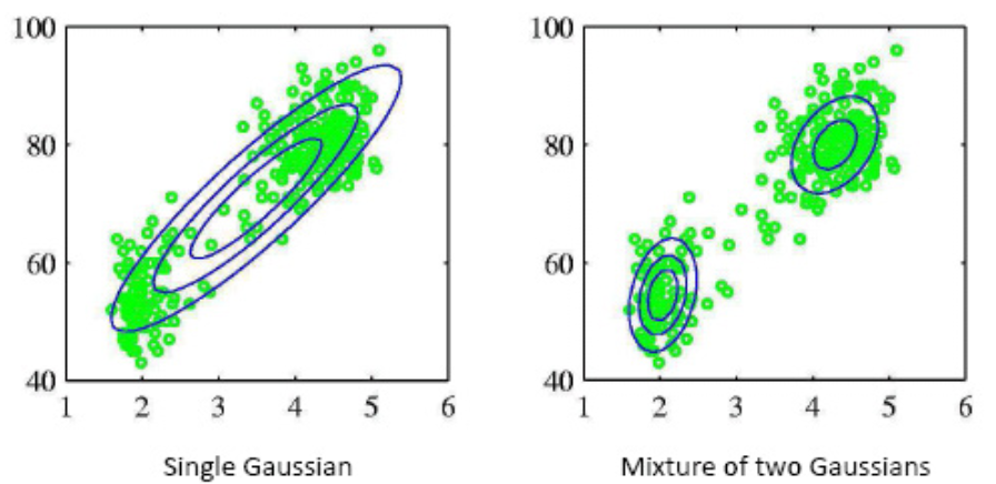
Fig. 133 Comparison of fitting with a single Gaussian and a mixture of two Gaussians.
Model
We assume there are \(K\) latent Gaussian components.
where \(\pi_k\) are mixing coefficients, which is the probability that \(\boldsymbol{x}\) is from class \(k\)
For instance, when \(K=3\), and \(\boldsymbol{x} \in \mathbb{R}\), then the mixture is like
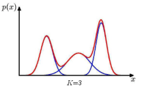
Fig. 134 A mixture of three univariate Gaussians
For bivariate cases,
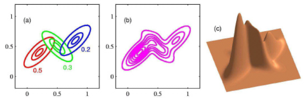
Fig. 135 A mixture of three bivariate Gaussians
Essentially any distribution can be approximated arbitrarily well by a large enough Gaussian mixture. But, maximum-likelihood estimation of parameters is not trivial.
Estimation
Given a data set and \(K\), let \(\boldsymbol{\theta} = (\boldsymbol{\mu} _1, \ldots, \boldsymbol{\mu} _k, \boldsymbol{\Sigma} _1, \ldots, \boldsymbol{\Sigma} _k)\), the log probability is
When \(K=1\), this becomes a single multivariate Gaussian problem which has a closed-form solution. But when \(K\ge 2\), there is no closed-form solution \(\boldsymbol{\pi}, \boldsymbol{\mu} _1, \boldsymbol{\mu} _2, \ldots, \boldsymbol{\mu} _K, \boldsymbol{\Sigma} _1, \boldsymbol{\Sigma} _2, \ldots \boldsymbol{\Sigma} _K\).
Introduce \(z_{ik}\)
For each observation \(i\), we introduce a set of binary indicator variables \(\boldsymbol{z}_i = z_{i 1}, \ldots, z_{i K}\) where \(z_{ik}=1\) if \(\boldsymbol{x}_i\) came from Gaussian component \(k\) and \(z_{ik}=0\) otherwise.
If we know \(\boldsymbol{z}_i\), then we can obtain the ML estimates of the Gaussian components just like in the single-Gaussian case:
\[\begin{split} \begin{aligned} \hat{\boldsymbol{\mu}}_{k} &=\frac{1}{n_{k}} \sum_{i=1}^{n} z_{i k} \boldsymbol{x}_i \\ \widehat{\boldsymbol{\Sigma} }_{k} &=\frac{1}{n_{k}} \sum_{i=1}^{n} z_{i k}\left(\boldsymbol{x}_i -\hat{\boldsymbol{\mu}}_{k}\right)\left(\boldsymbol{x}_i -\hat{\boldsymbol{\mu}}_{k}\right)^{\top} \\ \hat{\pi}_{k} &=\frac{n_{k}}{n} \end{aligned} \end{split}\]If we known the parameters, then the posterior probability of the indicator variables is
\[ \gamma_{i k}=\mathbb{P} \left(z_{i k}=1 \mid \boldsymbol{x}_{i}, \boldsymbol{\theta} \right)=\frac{{\pi}_{k} \operatorname{\mathcal{N}} \left(\boldsymbol{x}_{i} \mid {\boldsymbol{\mu}} _{k}, {\boldsymbol{\Sigma}} _{k}\right)}{\sum_{l=1}^{K} {\pi}_{\ell} \operatorname{\mathcal{N}} \left(\boldsymbol{x}_{i} \mid {\boldsymbol{\mu}} _{\ell}, {\boldsymbol{\Sigma}} _{\ell}\right)} \]where \(\gamma_{ik}\) is called the responsibility of the \(k\)-th component for \(\boldsymbol{x}_i\). Note that \(\sum_{k=1}^{K} \gamma_{i k}=1\)
Then we “pretend” that the \(\gamma_{ik}\) are the indicator variables themselves, and compute \(n_{k}=\sum_{i=1}^{n} \gamma_{i k}\) (may not be integer). We can then re-estimate the ML estiamtes by substituting \(z_{ik}\) by \(\gamma_{ik}\).
\[\begin{split} \begin{aligned} \hat{\boldsymbol{\mu}}_{k} &=\frac{1}{\sum_{i=1}^{n} \gamma_{i k}} \sum_{i=1}^{n} \gamma_{i k} \boldsymbol{x}_{i} \\ \hat{\boldsymbol{\Sigma}}_{k} &=\frac{1}{\sum_{i=1}^{n} \gamma_{i k}} \sum_{i=1}^{n} \gamma_{i k}\left(\boldsymbol{x}_{i}-\hat{\boldsymbol{\mu}}_{k}\right)\left(\boldsymbol{x}_{i}-\hat{\boldsymbol{\mu}}_{k}\right)^{\top} \\ \hat{\pi}_{k} &=\frac{\sum_{i=1}^{n} \gamma_{i k}}{n} \end{aligned} \end{split}\]
In reality, we know neither the parameters nor the indicators
EM algorithm
By introducing \(z_{ik}\), we would like to maximize the complete data likelihood
or its log
It can be shown that we are actually maximizing its expectation w.r.t. \(\boldsymbol{z}\)
Motivated from the above analysis, we can come up with the expectation-maximization algorithm.
Here comes the expectation-maximization (EM) algorithm
Initialization: Guess \(\boldsymbol{\pi}, \boldsymbol{\theta}\)
Iterate:
E-step: Compute \(\gamma_{ik}\) using current estimates of \(\boldsymbol{\pi}, \boldsymbol{\theta}\)
M-step: Estimate new parameters \(\boldsymbol{\pi}, \boldsymbol{\theta}\), by maximizing the expected likelihood, given the current \(\gamma_{ik}\)
Until log likelihood converges
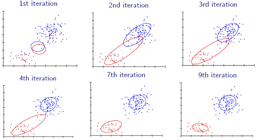
Fig. 136 Iterations of EM algorithms [Livescue 2021]
Regularization
If an initial guess of cluster center \(\boldsymbol{\mu}\) happens to be close to some data point \(\boldsymbol{x}\) and the variance is happen to be small, then the ML over \(\boldsymbol{x}\) is very large, i.e. overfitting.
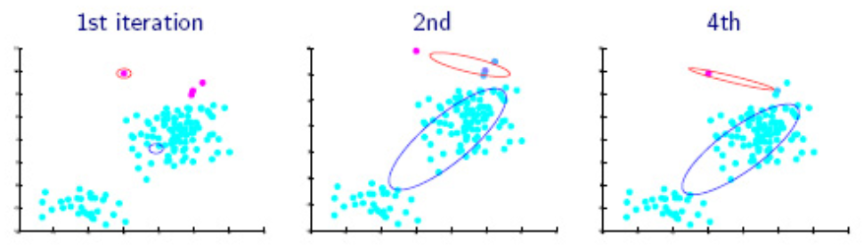
Fig. 137 Gaussian mixture fails if initialized at a point
Solutions
Start with large variance, and put lower bound of variance on each dimension of each component in the iterations.
Try several initialization and pick the best one. Best can be measured by some metrics, e.g. minimum entropy, maximum purity.
Held-out data
Instead of maximizing the expected likelihood in the M-step, maximize the posterior probability of \(\theta\) (MAP estimate).
\[\boldsymbol{\theta}=\underset{\boldsymbol{\theta}}{\operatorname{argmax}} \mathbb{E} _{\boldsymbol{z} \mid \boldsymbol{X}, \boldsymbol{\pi} , \boldsymbol{\theta}}[\ln p(\boldsymbol{X} , \boldsymbol{Z} \mid \boldsymbol{\pi}, \boldsymbol{\theta})]+\ln p(\boldsymbol{\theta} )\]
Model Selection (\(K\))
Straw man idea: Choose \(K\) to maximize the likelihood
Result: A separate, tiny Gaussian for each training example
In the limit \(\Sigma \rightarrow 0\), this yields infinite likelihood
Consider the number of parameters in a Gaussian mixture model \(\mathcal{M}\) with \(K\) components and dimensionality \(D\):
We need penalty on large \(d(\mathcal{M})\). Below are some terms often used to compare model complexity
Bayesian Information Criterion (BIC): Learn a model for each K that optimizes the likelihood L(M), then choose the model that maximizes
\[ \operatorname{BIC} (\mathcal{M})=L(\mathcal{M})-\frac{d(\mathcal{M})}{2} \log n \]Akaike information criterion (AIC), minimum description length (MDL), etc.
In practice,
most often use cross-validation to choose hyper-parameters like \(K\) or the minimum variance.
start from small \(K\) and growing
Start with a single Gaussian, do EM until convergence
Repeat: Split each Gaussian into two Gaussians with slightly different means, run EM, test on development set
Until no performance improvement on development set
Remarks
Any skewed sampling distribution, even slightly, can fit to several small mixtures towards the tail, even if the distribution actually is not a mixture.
There should be good reasons to belief that the underlying distribution is a mixture, before fitting the model.
A typical or common situation: There are two obvious humps, but a three-component mixture models fits much better than an obvious two-component one. The third component is small but connects the two larger ones well.
Mixture of normal components with covariance \(\boldsymbol{\Sigma} _i = \sigma^2 \boldsymbol{\Sigma}\) is approximately the same as K-means.