Semi-supervised Learning
(Figure credits: Jerry Zhu ICML 2007 tutorial unless otherwise indicated)
We often have access to a small amount of labeled data plus a large amount of unlabeled data.
Why not just get more labeled data?
Some labeled data is easy to get more of, e.g. tagged images
Some is expensive/time consuming/difficult/unethical to get:
Medical measurements (e.g. scans, neural recordings)
Phonetic transcription of speech: roughly 400x real time, requires experts
Text parsing: takes years to collect a few 1000 sentences’ worth
We introduce semi-supervised learning techniques for classification tasks.
Notions:
Input \(x\), label \(y\)
Function to be learned: \(f:\mathcal{X} \rightarrow \mathcal{Y}\)
Labeled data of size \(\ell\): \((\mathcal{X}_\ell, \mathcal{Y}_\ell) = \left\{ (x_{1:\ell}, y_{1:\ell}) \right\}\)
Unlabeled data \(\mathcal{X}_u = \left\{ x_{\ell + 1:n} \right\}\), where \(\ell \ll n\)
Test data \(\mathcal{X}_{test} = \left\{ x_{n+1:} \right\}\)
If we have labeled data, how can unlabeled data help?
Unlabeled data tells us something about the distribution of the data, and therefore where “reasonable” class boundaries may be.
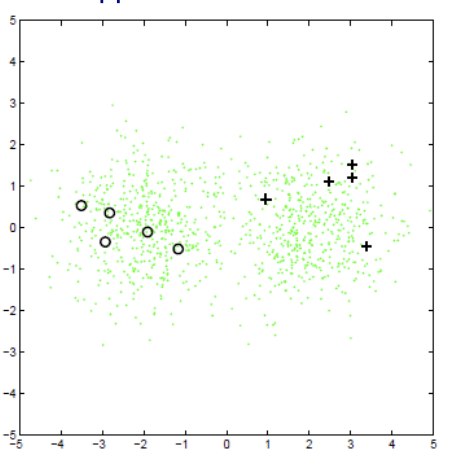
Fig. 39 Unlabeled data tells us about the “true” boundary.
Types of Semi-sup Learning
Transductive learning
Goal is to label the unlabeled training data (only. not necessary learn a labeling function). Aka label propagation.
Inductive learning (semi-supervised learning)
Goal is to learn a function that can be applied to new test data.
Weak labels/distant supervision
We have labels, but they are not exactly for the target task.
pairs from “Same/different” class, instead of class labels
subset of latent variables labeled but not all (e.g. object category in an image, but not boundaries of that object)
“downstream” labels (e.g. click-through counts instead of search result correctness)
Pre-training
Pre-train representation of unlabeled data, and use that representation along with the labeled data to learn a predictor.
For instance,
train PCA using unlabeled data \(\mathcal{X}_u\)
use the trained PCA to obtain representation \(\mathcal{Z}_\ell\) of labeled data \(\mathcal{X} _\ell\)
use \(\mathcal{Z}_\ell\) and \(\mathcal{Y}_\ell\) to train SVM.
Multi-task learning
Add an unlabeled loss term to a labeled loss.
Self-training
Algorithm
Train classifier \(f\) over labeled data \(\left( \mathcal{X} _\ell, \mathcal{Y} _\ell \right)\)
Predict on some unlabeled data \(x_u \in \mathcal{X}_u\)
Augmentation: Add some \((x_u, f(x_u))\) to labeled data set such that \(\left( \mathcal{X}_\ell \cup \left\{ x_u \right\} _\ell, \mathcal{Y} _\ell \cup \left\{ f(x_u) \right\} \right)\).
Repeat
Note that
This is a type of “wrapper” technique: can be used with any type of learning algorithm for \(f\).
Typically, only \((x_u, f(x_u))\) pairs with high confidence (e.g. probability) are used.
Pros and Cons
Pros
Very simple
A “wrapper” method: Can be applied with any existing classifier
Has had some real-world successes (e.g. in speech recognition)
Cons
Very risky: Can easily diverge if some early mistakes are made such that the augmented labeled set is contaminated.
Little theoretical understanding
Semi-supervised Generative Models
Labeled Data Only
Suppose the labeled data are categorical. We can then train a generative model, with one Gaussian per class. That is, for each class, the generative model is
Which can be trained by maximum likelihood (closed-form solution).
In prediction, for a new data point \(x_{\text{test} }\), we classify by finding the label with maximum probability \(p(y \mid x_{\text{test} }, \theta)=\frac{p(x_{\text{test} }, y \mid \theta)}{\sum_{y^{\prime}} p\left(x_{\text{test} }, y^{\prime} \mid \theta\right)}\).
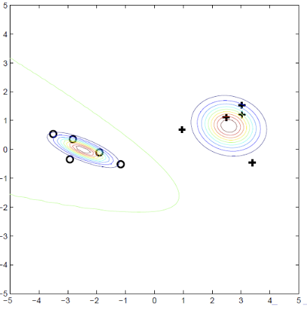
Fig. 40 Train a Gaussian for each class
Available Unlabeled Data
Suppose now we have unlabeled data as below. Clearly, the classifier boundaries above are not accurate.
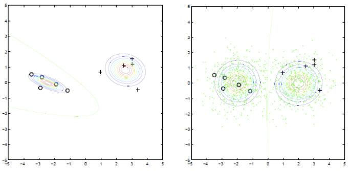
Fig. 41 Labeled and unlabeled data.
To improve it, we can do MLE using both labeled and unlabeled data. The joint log-likelihood is
where on RHS
the first term is log-likelihood for labeled data
the second term is log-likelihood for unlabeled data, assume it from mixtures Gaussian.
Now we have hidden variables (labels of \(x_u\)), so we can use EM. Same as EM for general Gaussian mixture learning, but some of the latent variables (component assignments) are hard labels while the rest are posteriors (as usual).
This method
Can be applied to other generative models, e.g. hidden Markov models (speech, text, video, other time series)
Amounts to doing EM for the appropriate model, treating unseen labels as latent variables.
cf. Gaussian Mixtures
Gaussian mixtures are clustering models. Given \(\mathcal{X} _u\), and number of class, say \(k\), then we can train Gaussian mixtures to learn \(k\) distribution functions for \(\mathcal{X} _u\). However, we don’t know the mapping from cluster index to the class index – given a new data point \(x_{\text{test} }\), we cannot do classification.
Labeled data help to find such mapping.
Pros and Cons
Semi-supervised generative models inherit many of the qualities of generative models
If the model is a good fit to the data, can be very effective
Provides an intuitive, clear probabilistic interpretation
But, doesn’t work well if we don’t have an accurate generative model for the unlabeled data
And, sometimes we’d rather classify with a non-generative model
Cluster-then-label
Clustering techniques can be used for classification. Suppose there are \(k\) categories. Algorithms are:
Cluster all labeled and unlabeled features \(\mathcal{X} _\ell \cup \mathcal{X} _u\) to \(k\) clusters.
For each proposed cluster, we need to find a mapping to the true class. One greedy method is to find the majority label in that cluster.
This makes fewer assumptions about the data distribution (unlike generative models), but also more unstable.
Graph-based Algorithms
Some data don’t fit simple generative models, and more complex generative models are hard to learn. We can use graph-based algorithms. Here we introduce a label propagation algorithm via random walk.
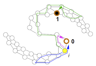
Fig. 42 An example of graph-based labeled and unlabeled data.
Like graph-based dimensionality reduction methods, we create an induced graph from the data set. Assume binary data. The algorithm is
Start from any node \(i\) and walk to node \(j\) with probability \(\frac{w_{ij}}{\sum _{k \in N(i)} w_{ik}}\)
Repeat until walk to a labeled node
Repeat many times, and the probability of hitting a label-1 node is regarded as the posterior probability of class 1 for node \(i\).
Another method to compute this probability value is
Initialize \(f(x_i)=y_i\) for labeled nodes, and 0 for unlabeled nodes
For all unlabeled nodes \(i\), update \(f(x_{i})=\frac{\sum_{j \in N(i)} w_{i j} f\left(x_{j}\right)}{\sum_{j \in N(i)} w_{i j}}\). Repeat until convergence.
Essentially, at each iteration, we take the weighted average over the neighbors.
The \(f(\cdot)\) values can alternatively be computed via an eigenproblem on the graph Laplacian.
Pros and Cons
Pros
Better than graph-based cluster-then-label method since it consider labels into the loss function.
Cons
Transductive method, no out-of-sample prediction.
Some original labels might be wrong, or we might be dealing with outliers
Sols:
Allow labeled points to be “relabeled” with some penalty
Define a kernel that approximates the graph similarity
Taken together, these extensions are referred to as “manifold regularization”
For more details, see Zhu’s tutorial.
Multi-view Algorithms: Co-Training
[Blum & Mitchell 1998]
The feature vector can be naturally split into two views \(x = [x^{(1)} x^{(2)}]\). E.g., \(x^{(1)}=\) image pixels, \(x^{(2)} =\) text description. We train two classifiers, one for each view. The idea is: The two classifiers “supervise” each other; when one is unconfident, hopefully the other one is.
Assumptions
\(x^{(1)}\) or \(x^{(2)}\) alone suffices for good classification, given enough data
\(x^{(1)}\) and \(x^{(2)}\) are independent given the class label
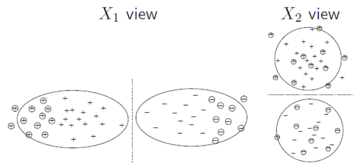
Fig. 43 Two views, each suffices for good classification, and independent of each other given the class label
Algorithm
Train two classifiers, \(f^{(1)}\) from \((\mathcal{X} ^{(1)}_\ell,\mathcal{Y} _\ell)\) and \(f^{(2)}\) from \((\mathcal{X} ^{(2)},\mathcal{Y} _\ell)\).
Classify two views of \(\mathcal{X} _u\) with each \(f^{(i)}\) separately
Add the \(k\) most-confident \((x_u,f^{(1)}(x_u))\) pairs to \(f^{(2)}\)’s labeled data
Add the \(k\) most-confident \((x_u,f^{(2)}(x_u))\) pairs to \(f^{(1)}\)’s labeled data
Repeat
Variants
Co-EM: Add all unlabeled data at each step, not just the top k, with some probability based on the confidence
Create multiple random (fake) feature splits (features are relevant but redundant)
Generalized multi-view
No feature split at all
Just train multiple classifiers of different types
Classify the unlabeled data with all of the classifiers
Add majority vote label
Pros and Cons
Advantage
Wrapper method: Can be wrapped around any existing classifier and learning algorithm
If the assumptions holds, it works very well
Has theoretical proof
Disadvantages
The assumptions are not often satisfied