Logistic Regression¶

Aka binomial GLM.

Logistic regression is used to model binary response \(Y_i \sim \operatorname{Ber}(p_i)\).

If we use OLS to model the binary response, we call this linear probability model (LPM)

\[\begin{split}\begin{aligned} Y_i &= \boldsymbol{x}_i ^\top \boldsymbol{\beta} + \varepsilon_i \\ \operatorname{E}\left( Y_i \right) &= \boldsymbol{x}_i ^\top \boldsymbol{\beta} \end{aligned}\end{split}\]

It is not appropriate since

Heteroskedasticity: \(\operatorname{Var}\left( Y_i \right) = p_i (1-p_i)\) where \(p_i\) depends on \(\boldsymbol{x}\)
Range: LHS is either \(1\) or \(0\), while RHS is in \(\mathbb{R}\).
Error and \(Y\) are negatively correlated.
Prediction: to predict a binary outcome, if predicted probability is larger than \(0.5\), then output 1, else 0

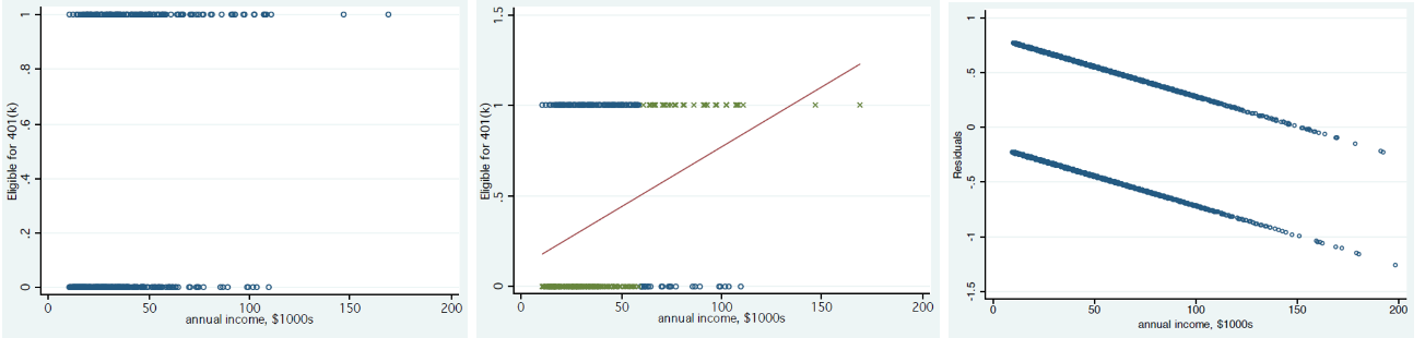
Fig. 73 Scatter plot (left) of binary \(Y\), fitted line with 0.5 cutoff for prediction (middle) and residual plot (right) if we fit OLS [Meyer 2021]¶

But rather than \(Y_i \sim \operatorname{Bin}(n_i, p_i)\), the book views \(n_{i}Y_{i}\sim\operatorname{Bin}(n_i, \pi_i)\), or \(Y_{i}\sim \frac{1}{n_i} \operatorname{Bin}(n_i, \pi_i)\) as random component, where \(Y_{i}\) is the proportion of success and \(\operatorname{E}(Y_i)=\pi_{i}\). It’s easier to define a link function as a function of \(\operatorname{E}(Y_i)\).

Data Structure¶

Logistic regression can take two types of data structure as input.

Ungrouped Data¶

For ungrouped data, suppose there are \(N\) observations, each observation \(y_{i}\) results from a single Bernoulli trial \(Y_{i}\sim\operatorname{Ber}(p_i)\) and equals 0 or 1.

A large-sample means \(N\rightarrow\infty\).

Note that for different \(i_{1}\ne i_{2}\), they may share the same covariates \(\boldsymbol{x}_{i_{1}}=\boldsymbol{x}_{i_{2}}\). So they share the same underlying expectation \(\pi_{i}\). Thus, we may consider group them together to obtain grouped data.

Grouped Data¶

Suppose there are \(n_{i}\) is the number of observations at setting \(i\) of the covariates, \(i=1, 2, \ldots, N\).

A large-sample means \(n_{i}\rightarrow\infty\) for every \(i\).

Warning

The two data types can be converted to each other. The MLE and the asymptotic distribution are the same since the log-likelihood differ by a constant.
However, the summary of fit, such as deviance, are not the same, since the saturated models are different.
The goodness-of-fit test for ungrouped data is invalid, since the saturated model for ungrouped data requires \(p=n\), but the distribution of test statistic is derived when \(p\) is fixed and \(n\rightarrow\infty\).

Model Structure¶

Derivation of Link Function¶

We have the random component \(Y_{i}\sim\frac{1}{n_{i}} \operatorname{Bin}( {n_{i}}, {\pi_{i}})\) and \(\operatorname{E}(Y_i)=\pi_{i}\). Now we want to find a link function \(g\) such that

\[ g(\pi_{i})=\boldsymbol{x}_{i}^{\top}\boldsymbol{\beta} \]

i.e.

\[ \pi_{i}=g^{-1}(\boldsymbol{x}_{i}^{\top}\boldsymbol{\beta}) \]

Thus \(g^{-1}\) is a function mapping from \(\mathbb{R}\) to \((0,1)\). Hence, it’s intuitive to consider a CDF.

Let \(g^{-1}=F\), where \(F\) is some CDF. Assume \(\epsilon_{i} \overset{\text{iid}}{\sim} F\). Then

\[ \pi_{i}=F(\boldsymbol{x}_{i}^{\top}\boldsymbol{\beta})=\operatorname{P} (\epsilon_{i}\le\boldsymbol{x}_{i}^{\top}\boldsymbol{\beta})=\operatorname{P}(0\le\boldsymbol{x}_{i}^{\top}\boldsymbol{\beta}-\epsilon_{i}) \]

We can define a latent variable \(Y_{i}^{*}=\boldsymbol{x}_{i}^{\top}\boldsymbol{\beta}-\epsilon_{i}\). Hence

\[ \pi_{i}=\operatorname{P}(Y_{i}^{*}\ge0) \]

If \(n_{i}=1\), then \(Y_{i}\) follows a binomial distribution

\[\begin{split} Y_{i}=\begin{cases} 1 & Y_{i}^{*}\ge0\\ 0 & Y_{i}^{*}<0 \end{cases} \end{split}\]

which means the observation of \(Y_{i}\) depends on the latent variable \(Y_{i}^{*}\). This kind of model is called a threshold model.

Some common choices of \(F\) are

Probit link: \(F\) is the CDF of \(N(0,1)\). That is, \(\pi_i = \Phi (\boldsymbol{x} _i ^\top \boldsymbol{\beta})\)

But the interpretation of \(\beta\) is not straightforward: One unit increase in \(X_j\) leads to \(\phi(\boldsymbol{x}_i ^\top \boldsymbol{\beta} )\beta_j\) increase in \(\pi_i\). We need to take derivative to compute the effect, and the effect also depends on values of current \(\boldsymbol{x}\).
- If we fix \(\boldsymbol{x}\) at sample mean \(\boldsymbol{\mu} _x\), then the computed effect is called partial effect at the average (PEA).
- If we compute the effect for each observation \(\boldsymbol{x}_i\), and take the average, the computed effect is called average partial effect (APE), which is preferred over PEA.
Logit link: \(F\) is the CDF of a logistic distribution

\[F(z)=\frac{1}{1+e^{-z}}\]

and \(g=F^{-1}\) is called a logit function

\[ g(\pi_{i})=\log\left(\frac{\pi_{i}}{1-\pi_{i}}\right)=\text{logit}(\pi_{i})=\boldsymbol{x}_{i}^{\top}\boldsymbol{\beta} \]

The logit link is the canonical link of the Binomial distribution
Log-log link: see book Section 5.6.3

Therefore, choosing logit link, our model is

\[\log\left(\frac{\pi_{i}}{1-\pi_{i}}\right)=\boldsymbol{x}_{i}^{\top}\boldsymbol{\beta}\]

where \(\pi_i = \operatorname{E}\left( Y_i \right)\).

Interpretation of \(\boldsymbol{\beta}\) as Odds Ratio¶

Suppose we use logit link and \(x_{j}\) increases 1 unit. Let \(p_{0}\) be the original probability and \(p_{1}\) be the updated probability, then

\[ \log\left(\frac{p_{1}}{1-p_{1}}\right)-\log\left(\frac{p_{0}}{1-p_{0}}\right)=\Delta\boldsymbol{x}_{i}^{\top}\boldsymbol{\beta}=\beta_{j} \]

i.e.

\[ e^{\beta_{j}}=\frac{p_{1}/(1-p_{1})}{p_{0}/(1-p_{0})} \]

The quantity \(p_{1}/(1-p_{1})\) is called an odds. And the ratio of two odds is called an odds ratio.

Thus, the interpretation is: the odds multiplies by \(e^{\beta_{j}}\) per unit increase in \(x_{j}\).

Estimation¶

Score Equations¶

Recall the general score equations are

\[ \sum_{i=1}^{N}\frac{\left(y_{i}-\mu_{i}\right)x_{ij}}{\operatorname{Var}\left(Y_{i}\right)}\frac{\partial\mu_{i}}{\partial\eta_{i}}=0,\quad j=1,2,\dots,p \]

Now in binary GLM, \(Y_{i}\sim\frac{1}{n_{i}}\operatorname{Bin} ({n_{i}},{\pi_{i}})\)

\(\operatorname{Var} (Y_{i})=\pi_{i}\left(1-\pi_{i}\right)/n_{i}\)
\(\operatorname{E}(Y_i)=\pi_{i}=\mu_{i}=F(\eta_{i})\)
\(\frac{\partial\mu_{i}}{\partial\eta_{i}}=\frac{\partial F(\eta_{i})}{\partial\eta_{i}}=f(\eta_{i})\)

The equations become

\[ {\sum_{i=1}^{N}\frac{n_{i}\left(y_{i}-\pi_{i}\right)x_{ij}}{\pi_{i}\left(1-\pi_{i}\right)}f\left(\eta_{i}\right)=0,\quad j=1,2,\ldots,p} \]

If we use canonical link, then

\[ {F(z)=\frac{e^{z}}{1+e^{z}},\quad f(z)=\frac{e^{z}}{\left(1+e^{z}\right)^{2}}=F(z)[1-F(z)]} \]

In addition, we have \(\pi_{i}=F(\eta_i)\). Hence, \(f(\eta_i) = \pi_i (1-\pi_i)\), and the equations simplify to

\[ {\sum_{i=1}^{N}n_{i}\left(y_{i}-\pi_{i}\right)x_{ij}=0,\quad j=1,\ldots,p} \]

which is

\[ \sum_{i=1}^{N}n_{i}y_{i}x_{ij}=\sum_{i=1}^{N}n_{i}\pi_{i}x_{ij} \]

That is, the score equations equate the sufficient statistics to their expected values.

Covariance of MLE¶

Applying the general formula,

\[ \text{Var}(\hat{\boldsymbol{\beta}})=\left[\boldsymbol{X}^{\top} \boldsymbol{W} \boldsymbol{X} \right]^{-1}=\left[\boldsymbol{X}^{\top}\boldsymbol{V} \boldsymbol{X} \right]^{-1}=\left[\boldsymbol{X}^{\top}\text{diag}(n_{i}\pi_{i}(1-\pi_{i})) \boldsymbol{X} \right]^{-1} \]

To estimate it, plug in \(\hat{\pi}_{i}\).

Computation¶

For logistic regression, Newton’s method = Fisher scoring = IRLS. (Section 5.4.1)

Note that some or all ML estimates may be infinite or may not even exist. See infinite parameter estimate.

Comparison¶

We can compare linear probability model, probit, and logit: how do the estimate the effect of a variable \(X\) on the binary response \(Y\)? Of course, the coefficient values are different, but,

Same sign
Roughly same significance
Roughly same out-of-sample prediction accuracy

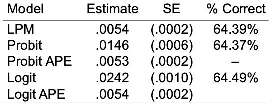
Fig. 74 Comparison of estimate in different models for binary response¶

Hypothesis Testing¶

Wald Test Disadvantages¶

First, its results depend on the scale for parameterization. Logit-scale statistic is too conservative and the proportion-scale statistic is too liberal.
Second, when a true probability in a binary regression model is very large, the Wald test is less powerful than the other methods and can show aberrant behavior, e.g. smaller p-value for stronger evidence.

Better use likelihood ratio test or score test.

Deviance¶

Note again that the goodness-of-fit test for ungrouped data is invalid, since the saturated model for ungrouped data requires \(p=n\) but the distribution of test statistic is derived when \(p\) is fixed and \(n\rightarrow\infty\).

The deviance comparing a fit \(\hat{\boldsymbol{\pi}}\) v.s. the saturated model is

\[\begin{split} \begin{aligned} D(\boldsymbol{y},\hat{\boldsymbol{\pi}}) & = - 2\left[\ell(\hat{\boldsymbol{\mu}}\vert\boldsymbol{y})-\ell(\tilde{\boldsymbol{\mu}}\vert\boldsymbol{y})\right] \\ &= -2\log\left\{ \left[\prod_{i=1}^{N}\hat{\pi}_{i}^{n_iy_i}\left(1-\hat{\pi}_{i}\right)^{n_{i}-n_{i}y_{i}}\right]/\left[\prod_{i=1}^{N}y_{i}^{n_{i}y_{i}}\left(1-y_{i}\right)^{n_{i}-n_{i}y_{i}}\right]\right\} \\ &=2\sum_{i}n_{i}y_{i}\log\frac{n_{i}y_{i}}{n_{i}\hat{\pi}_{i}}+2\sum_{i}\left(n_{i}-n_{i}y_{i}\right)\log\frac{n_{i}-n_{i}y_{i}}{n_{i}-n_{i}\hat{\pi}_{i}} \end{aligned}\end{split}\]

Thus, the deviance is a sum over the \(2N\) success and failure totals at the \(N\) settings, which satisfies the general form

\[ {D(\boldsymbol{y},\hat{\boldsymbol{\mu}})=2\sum}\text{observed}{\times\log\left(\frac{\text{ observed }}{\text{fitted }}\right)} \]

Note

The words observed and fitted here means counts, not proportion.
For grouped data, the saturated model has a parameter at each \(\boldsymbol{x}_i\) setting for the explanatory variables. For ungrouped data, by contrast, it has a parameter for each subject \(i\).

Pearson Statistic¶

It is also the sum over \(2N\) cells of successes and failures.

\[\begin{split} {\begin{aligned}X^{2} & =\sum_{i=1}^{N}\frac{\left(n_{i}y_{i}-n_{i}\hat{\pi}_{i}\right)^{2}}{n_{i}\hat{\pi}_{i}}+\sum_{i=1}^{N}\frac{\left[\left(n_{i}-n_{i}y_{i}\right)-\left(n_{i}-n_{i}\hat{\pi}_{i}\right)\right]^{2}}{n_{i}\left(1-\hat{\pi}_{i}\right)}\\ & =\sum_{i=1}^{N}\frac{\left(n_{i}y_{i}-n_{i}\hat{\pi}_{i}\right)^{2}}{n_{i}\hat{\pi}_{i}\left(1-\hat{\pi}_{i}\right)}\\ & =\sum_{i=1}^{N}\frac{\left(y_{i}-\hat{\pi}_{i}\right)^{2}}{\hat{\pi}_{i}\left(1-\hat{\pi}_{i}\right)/n_{i}} \end{aligned} } \end{split}\]

It satisfies the general form

\[ X^{2}=\sum\frac{(\text{ observed }-\text{ fitted })^{2}}{\text{ fitted }} \]

Note

The words observed and fitted here means counts \(n_{i}y_{i}\), not proportion \(y_{i}\). If you substitute observed value of \(y_{i}\) and fitted value \(\hat{y}_{i}\), like Poisson GLM, then you are wrong. However, in the last equality satisfying the form \(\sum\frac{(y_{i}-\mu_{i})^{2}}{v(\mu_{i})}\), \(y_{i}\) is proportion, not counts. So we see the notation \(Y_{i}\sim\frac{1}{n_{i}}\operatorname{Bin} ({n_{i}},{\pi_{i}})\) is very disgusting.
Though the form \(\sum\frac{(\text{ observed }-\text{ fitted })^{2}}{\text{ fitted }}\) is very succinct, the support of the summation is not specified. One may think the support is \(1, 2, \ldots, N\), but here the summation is over \(2N\) cells of successes and failures. It will be more easy to understand this if we regard binomial distribution as a multinomial distribution with \(c=2\).

Infinite Parameter Estimate¶

One may sometimes see this warning message using R to solve the logistic regression:

\[ \texttt{Warning message: glm.fit: fitted probabilities numerically 0 or 1 occurred} \]

You may see very large estimates of \(\boldsymbol{\beta}\). What happened?

Suppose the data is ungrouped, where \(y_{i}=0\) or \(1\).

Complete Separation / Perfect Discrimination¶

Suppose there exists \(\boldsymbol{\beta}_{s}\) such that if \(\boldsymbol{x}_{i}^{\top}\boldsymbol{\beta}_{s}>0\) then \(y_{i}=1\) otherwise \(y_{i}=0\), i.e. a hyperplane perfectly separate two types of points.

If we let \(\boldsymbol{\beta}=k\boldsymbol{\beta}_{s}\), as \(k\rightarrow\infty\),

\[\begin{split} \pi_{i}=\frac{1}{1+e^{-\boldsymbol{x}_{i}^{\top}\boldsymbol{\beta}}}\rightarrow\begin{cases} 1 & \boldsymbol{x}_{i}^{\top}\boldsymbol{\beta}_{s}>0, \text{i.e.}, y_i = 1 \\ 0 & \boldsymbol{x}_{i}^{\top}\boldsymbol{\beta}_{s}<0, \text{i.e.}, y_i = 0 \end{cases} \end{split}\]

Substituting this \(\pi_{i}\) into the score function gives

\[ \frac{\partial\ell}{\partial\beta_{j}}=\sum_{i}(y_{i}-\pi_{i})x_{ij}\rightarrow 0\text{ for all }j \]

which means the infinite estimate \(\boldsymbol{\beta}=k\boldsymbol{\beta}_{s}\rightarrow\infty\) is a solution to the score function.

Indications include

The reported log-likelihood value is 0 to any decimal places
standard errors are unnaturally large.

Quasi-complete Separation¶

Suppose there exists \(\boldsymbol{\beta}_{s}\) such that

if \(\boldsymbol{x}_{i}^{\top}\boldsymbol{\beta}_{s}>0\) then \(y_{i}=1\)
if \(\boldsymbol{x}_{i}^{\top}\boldsymbol{\beta}_{s}<0\) then \(y_{i}=0\)
if \(\boldsymbol{x}_{i}^{\top}\boldsymbol{\beta}_{s}=0\) then \(y_{i}=0\) or \(1\)

i.e. we allow both types of data points lie on the separation hyperplane. Then at least one estimate is infinite.

Let \(\boldsymbol{\beta}=k\boldsymbol{\beta}_{s}+\left(\begin{array}{c} \beta_{0}\\ \boldsymbol{0} \end{array}\right)\), where \(\beta_{0}\) is a scalar added to the intercept. Then as \(k\rightarrow\infty\),

\[\boldsymbol{x}_{i}^{\top}\boldsymbol{\beta}=\boldsymbol{x}_{i}^{\top}(k\boldsymbol{\beta}_{s})+\beta_{0}\rightarrow\infty\]

for \(\boldsymbol{x}_{i}^{\top}\boldsymbol{\beta}_{s}\ne 0\). Hence

\[\begin{split} {\pi_{i}=\frac{1}{1+e^{-\boldsymbol{x}_{i}^{\top}\boldsymbol{\beta}}}\rightarrow\left\{ \begin{array}{ll} 1 & \text{ if }\boldsymbol{x}_{i}^{\top}\boldsymbol{\beta}_{s}>0\\ 0 & \text{ if }\boldsymbol{x}_{i}^{\top}\boldsymbol{\beta}_{s}<0\\ \frac{e^{\beta_{0}}}{1+e^{\beta_{0}}} & \text{ if }\boldsymbol{x}_{i}^{\top}\boldsymbol{\beta}_{s}=0 \end{array}\right.} \end{split}\]

The score function for \(\beta_{j}\) is

\[ \frac{\partial\ell}{\partial\beta_{j}}=\sum_{i}(y_{i}-\pi_{i})x_{ij}\rightarrow\sum_{i\vert\boldsymbol{x}_{i}^{\top}\boldsymbol{\beta}_{s}=0}\left(y_{i}-\frac{e^{\beta_{0}}}{1+e^{\beta_{0}}}\right)x_{ij} \]

Equating it to 0 gives

\[ \frac{\sum_{i\vert\boldsymbol{x}_{i}^{\top}\boldsymbol{\beta}_{s}=0}y_{i}x_{ij}}{\sum_{i\vert\boldsymbol{x}_{i}^{\top}\boldsymbol{\beta}_{s}=0}x_{ij}}=\frac{e^{\beta_{0}}}{1+e^{\beta_{0}}} \]

so we can solve for \(\beta_{0}\).

This means that, \(\beta_{j}\rightarrow\infty\) is a solution to the \(j\)-th score equation. How about other score equations?

Indications include

The reported log-likelihood value is less than 0
standard errors are unnaturally large.

Remedy¶

Inference such as likelihood ratio test, confidence interval are possible. With quasi-complete separation, some parameter estimates and SE values may be unaffected, and even Wald inference methods are available with them.

To make estimtes finite, approches include smoothing the data, and maximizes a penalized likelihood function.

Application: Case-Control Study¶

In some study, researchers want to find the effect of \(X\) on \(Y\). Say, \(Y\) is lung cancer and \(X\) is smoking. There are two kinds of study design

Prospective design: randomized experiment. Randomly select smokers and non-smokers from the population and observe whether they will develop cancer in the future.
- We can compare \({\mathbb{E}(Y=1|X=1)}\text{ with }{\mathbb{E}(Y=1|X=0)}\)
- Cons: takes time; lung cancer is a rare disease, may observe very few cancer
Case-control study (retrospective): We randomly select some samples from patients who develop cancer and some samples from healthy controls. Then, we check whether the person has been a smoker or not
- Now we can only compare \({\mathbb{E}(X=1|Y=1)}\) with \({\mathbb{E}(X=1|Y=0)}\)
- The study takes a shorter time, and we can obtain enough cancer cases

Can we do case-control study to estimate some quantities in prospective study? Note that from the formula of conditional probability, we have

\[\begin{split} {\begin{aligned}\mathrm{OR} & =\frac{\mathbb{P}(Y=1|X=1)/\mathbb{P}(Y=0|X=1)}{\mathbb{P}(Y=1|X=0)/\mathbb{P}(Y=0|X=0)}\\ & =\frac{\mathbb{P}(X=1|Y=1)/\mathbb{P}(X=0|Y=1)}{\mathbb{P}(X=1|Y=0)/\mathbb{P}(X=0|Y=0)} \end{aligned} } \end{split}\]

Even if we include other covariates, this also holds

\[\begin{split} \begin{aligned} {OR\vert_{\tilde{X}=x}} & =\frac{\mathbb{P}(Y=1|X=1,\tilde{X}=x)/\mathbb{P}(Y=0|X=1,\tilde{X}=x)}{\mathbb{P}(Y=1|X=0,\tilde{X}=x)/\mathbb{P}(Y=0|X=0,\tilde{X}=x)}\\ & =\frac{\mathbb{P}(X=1|Y=1,\tilde{X}=x)/\mathbb{P}(X=0|Y=1,\tilde{X}=x)}{\mathbb{P}(X=1|Y=0,\tilde{X}=x)/\mathbb{P}(X=0|Y=0,\tilde{X}=x)}\\ & =e^{\beta_{X}} \end{aligned} \end{split}\]

Thus, building the logistic regression using case-control study samples is the same as building the model using prospective samples.