K-nearest neighbors
\(K\)-nearest neighbors is a non-parametric method. It simply the application of nearest-neighbor smoothing on a graph.
It can be used for both classification and regression. The nearest-neighbor methods can also be applied to a graph with vertex attributes.
Classification from Data Matrix
If the input is a data matrix, \(K\)-nearest neighbors method look at the \(K\) points in the training set \(\mathcal{D}\) that are nearest to the test input \(\boldsymbol{x}_i\), denoted \(N_K \left( \boldsymbol{x}_i, \mathcal{D} \right)\). To define ‘nearest’, it requires a distance measure \(d(\boldsymbol{x}_i, \boldsymbol{x}_j)\), such as Euclidean distance.
To predict the class of observation \(\boldsymbol{x}\), use
Validation data is used to decide the hyper-parameter \(K\).
Regression on Graph
If the input is a graph \(G=(V, E)\) with vertex attribute \(x _v\), then for new vertex \(i\) with unknown attribute but known edges, we can predict its attribute value by the average of those of its neighbors,
Note that there is no hyper-parameter \(K\).
Tuning
To choose optimal \(K\), we can use train-test split.
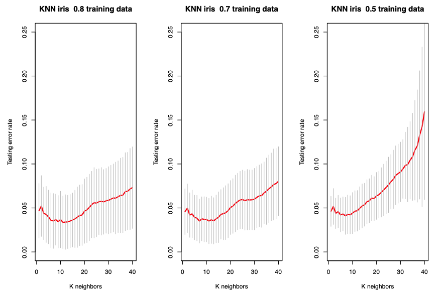
Fig. 80 Random train-test split for different ratios [Wang 2021]
As \(K\) increases from 1, the test error first decreases and then increases. The error bound increases.
Pros
Can express complex, non-linear, non-parametric boundaries
Very fast training
Simple, yet with good performance in practice
Reasonably good interpretability
Cons
It is an example of memory-based learning or instance-based learning. It stores all seen points.
Not among the best classifiers in terms of accuracy
Standardization is often necessary
Poor performance in high dimensional settings
In the graph case, how best to evaluate may not be clear in the case where \(\boldsymbol{x} _j\) is not observed for one or more \(j \in N_i\).
One solution to this dilemma is to redefine it in terms of only those vertices \(j \in V_i\) that are both adjacent to \(i\) and for which \(\boldsymbol{x} _j\) is observed.
Alternatively, we might impute values for the unobserved \(\boldsymbol{x} _j\), substituting, for instance, the overall average \(\frac{1}{\left\vert V_{obs} \right\vert}\sum _{k \in V_{obs}} \boldsymbol{x} _k\)
Although neither of these approaches is entirely satisfactory, imputation is likely to work better in practice, particularly when the relative number of missing observations is not small