Stochastic Gradient Descent
In this section we talk stochastic gradient descent in detail. Recall the three general steps in stochastic gradient descent:
run forward propagation with \(\Theta^{(t-1)}\) to compute the loss \(\mathcal{L}\left(\boldsymbol{X} , \boldsymbol{y}; \Theta^{(t-1)}\right)\)
compute gradient via chain rule \(\boldsymbol{g}^{(t)}(\boldsymbol{X}, \boldsymbol{y})=\nabla_{\Theta} \mathcal{L}\left(\boldsymbol{X} , \boldsymbol{y}; \Theta^{(t-1)}\right)\)
update the model parameters \(\Theta^{(t)}=\Theta^{(t-1)}-\eta \boldsymbol{g}^{(t)}\)
Then we check for stopping criteria (convergence of loss / gradient, model performance, etc).
Why “Stochastic”
SGD differ from standard GD on how the gradient is computed.
Basic Gradient Descent
- Definition (Epoch)
An epoch is a single pass through the training set.
A single “iteration” \(t\) can be an epoch, which means we loop over examples (or in parallel) to compute the gradient \(\boldsymbol{g}^{(t)}\left(\boldsymbol{x}_{i}, y_{i}\right)\) for each observation \(i\) and use the average gradient to approximate the true gradient
Then we make a single update at the end of the epoch.
Assuming \(n\) is large, \(\boldsymbol{g}^{(t)}(X, Y)\) is a good estimate for gradient, but it costs \(O(n)\) to compute.
Stochastic Gradient Descent
Computing gradient on all \(n\) examples is expensive and may be wasteful: many data points provide similar information.
Instead, SGD randomly select one observation at a time. It estimates the gradient on the entire set by the gradient on a single example in an iteration \(t\).
Mini-batch Gradient Descent
Mini-batch gradient descent use a batch \(B\) of observations to estimate the sample gradient in an iteration. For some \(B \subset \left\{ 1,2,\ldots, n \right\},|B| \ll n\),
In each epoch, we shuffle data, partition into batches, and iterate over batches. In this case, each update over a mini-batch is counted as an iteration. The number of iterations in an epoch equals \(n/\left\vert B \right\vert\).
In theory, if computation power is not an issue, we should set \(\left\vert B \right\vert\) as large as possible. But in practice, people found there are some advantages of small \(\left\vert B \right\vert\). Using small \(\left\vert B \right\vert\) works like adding noise to the gradient, which brings regularization effect and make the trained model more robust. Usually \(\left\vert B \right\vert = 32, 64\) are used.
Nowadays, the term SGD often refers to batch GD.
Comparison
We can plot the contours of the loss value w.r.t. parameter \(\boldsymbol{\Phi}\), and plot the trajectory of \(\boldsymbol{\Phi}^{(t)}\) for GD, SGD and mini-batch GD. We can see
GD has the smoothest trajectory
SGD has the most tortuous trajectory
Batch GD is between the two. Increasing the batch size reduces the noise in gradient.
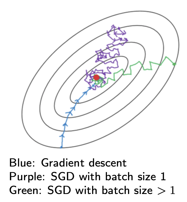
Fig. 160 Comparison of gradient descent methods [Shi 2021]
Learning Rate Scheduling
How to tune learning rate? First we review some concepts in optimization, and introduce learning rate decay, and finally introduce theoretical foundation for it.
Concepts Review
Local minimum
A point \(\boldsymbol{x}^{\&}\) where \(\boldsymbol{g}^{\&}=0\) and \(H^{\&}\succeq0\)
Stationary point
In classical optimization, \(x^{*}\) is a stationary point if the gradient is zero
\[ \nabla f(x^{*})=0 \]In deep learning SGD, gradient and parameter update and loss update are random since the batch is random
\[\begin{split} \begin{aligned} \hat{g} & =E_{(x,y)\sim\text{ Batch }}\nabla_{\Phi}\mathcal{L}(\Phi,x,y)\\ \Delta\Phi & =\eta\hat{g} \end{aligned} \end{split}\]Sometimes the stationary point \(\Phi^{*}\) is defined similarly as that in classical optimization, i.e. average gradient is zero
\[ \nabla_{\Phi}E_{(x,y)\sim\operatorname{Train}}\mathcal{L}(\Phi,x,t)=E_{(x,y)\sim\text{ Batch }}\nabla_{\Phi}\mathcal{L}(\Phi,x,y)=0 \]but sometimes we say we reach a stationary point \(\Phi^{*}\) of aloss function \(\mathcal{L}\) if that the (expected) loss update is 0, i.e.
\[ E\left[\mathcal{L}(\Phi^{*}+\Delta\Phi)-\mathcal{L}(\Phi^{*})\right]=0 \]
Stationary distribution
After we reach a stationary point, the parameters after one update is \(\Phi^{*}+\Delta_{1}\Phi\), after two update is \(\Phi^{*}+\Delta_{1}\Phi+\Delta_{2}\Phi\) and all these updated parameters follow a distribution \(\sim\) stationary distribution.
Learning Rate Decay
The magnitude of learning rate is important. When we are close to a minimum, if the learning rate is still large, then we will jump around and cannot achieve the minimum. Thus, an attempt is reduce learning rate by time.
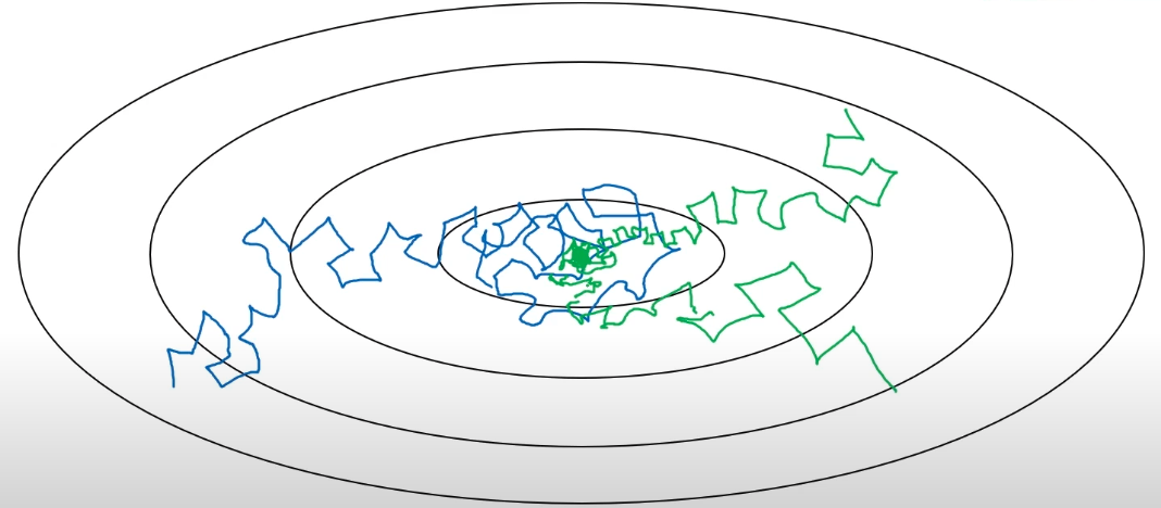
Fig. 161 Loss trajectory with (green) vs without (blue) learning rate decay [Ng 2017]
In practice, we start with a reasonable learning rate, and drop learning rate by some schedule
\(\eta = 0.95 ^{\text{epoch} } \eta_0\)
\(\eta = \frac{k}{\sqrt{\text{epoch}}} \eta_0\) or \(\eta = \frac{k}{\sqrt{t}} \eta_0\)
decay by a factor of \(\alpha\) every \(\beta\) epochs.
manually drop (typically 1/10) when loss appears stuck (monitor mini-batch training loss)
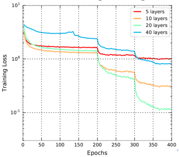
Fig. 162 Training loss drop down by learning rate decay [Shi 2021]
Classical Convergence Theorem
If use the fundamental update equation
and if the following conditions of learning rate holds
then
the training loss \(E_{(x,y)\sim\operatorname{Train}}\mathcal{L}(\Phi,x,t)\) will converges to a limit, and
any limit point of the sequence \(\Phi_{t}\) is a stationary point in the sense that the gradient at that point is \(0\).
\[ \nabla_{\Phi}E_{(x,y)\sim\operatorname{Train}}\mathcal{L}(\Phi,x,t)=0 \]
Note that it may be a saddle point, not a local optimum.
Optimizers
There are various algorithms to reduce oscillations in the training trajectory and speed up training.
Momentum SGD use a running average of gradient instead of the raw gradient.
RMSProp is an adaptive SGD methods, in the sense that they use different learning rates for different parameters.
Adam combines momentum and RMSProp, and is more widely used.
Momentum SGD
Momentum SGD use a running average of gradient instead of the raw gradient. The averaging step can reduce oscillations in the trajectory. It also has interpretation as velocity and acceleration.
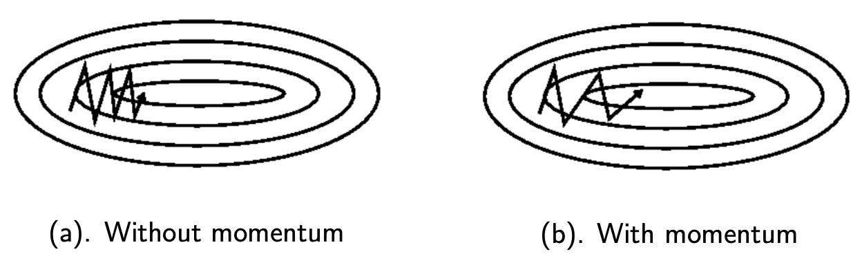
Fig. 163 SGD with and without momentum [S. Ruder]
Review of Running Average
First we review the concept of running average.
A running average \(\tilde{\boldsymbol{x}}_t\) on input \(x_t\) is written as a weight sum of previous value \(\tilde{\boldsymbol{x}}_{t-1}\) and new input \(x_t\)
or equivalently $\( \tilde{\boldsymbol{x}}_{t}=\beta\tilde{\boldsymbol{x}}_{t-1}+(1-\beta)x_{t} \)$
where $\( \beta=1-1/N \)$
Typical values for \(\beta\) are 0.9, 0.99 or 0.999 corresponding to \(N\) being \(10,100\) or \(1000\), which is the window size.
Bias correction in warm up period
Note there is a warm up period \(t<N\) of the running average \(\tilde{x}_{t}\), where the value is strongly biased toward zero if \(\tilde{x}_{0}=0\).
We can consider not to use the last \(N\) terms but use all other terms \(x_{1}\) to \(x_{t}\)
and we have \(\tilde{x}_{1}=x_{1}\), as initial value. But this fails to track a moving average when \(t\gg N\). So to combine the two methods together,
Algorithm
The standard momentum SGD algorithm is
where
\({\color{teal}{\boldsymbol{\tilde{g}}_{t}}}\) is a running average of gradient estimate \(\color{blue}{\hat{\boldsymbol{g}}_{t}}\), also interpreted as velocity
\(\color{blue}{\hat{\boldsymbol{g}}_{t}}\) is the gradient estimate, also interpreted as acceleration
\(N_g=10,100\) or \(1000\) is the window size.
The hyperparameters are \(N_g, \eta\).
Root Mean Square Prop (RMSProp)
Motivation
To reduce oscillations in the training trajectory, we wants to slow down learning in the parameter direction with large gradient, and speed up learning in the parameter direction with small gradient. To achieve this, we need parameter dimension-specific update, and a measure of large/small gradient in that parameter dimension.
One attempt is to can set the learning rate in the update equation \({\boldsymbol{\Phi}}_{t+1}[i]={\boldsymbol{\Phi}}_{t}[i]-\eta{\color{blue}{\hat{\boldsymbol{g}}_{t}[i]}}\) to be \(\eta_{i}=\eta_{0}/\sigma_{i}^{2}\), where \(\sigma_i^2 = \operatorname{Var}\left( \boldsymbol{g} _t[i] \right)\) is a measure of large/small gradient in that parameter dimension.
i.e. learning rate is inversely proportional to the variance.
But in practice, dividing by standard deviation works better
So question is, how to find \(\sigma _i\)?
Algorithm
RMSrPop’s approximates \(\sigma_i\) by a running average \(\boldsymbol{s}_{t}[i]\) of the second moment of the gradient of a particular parameter dimension, written as \({\color{blue}{\hat{\boldsymbol{g} }_{t}[i]^{2}}}\).
where \(\epsilon\) is used to avoid \(/0\).
Basically, \(\color{brown}{\boldsymbol{s}_{t}[i]}\) approximates the variance \(\operatorname{Var} (\color{blue}{\hat{\boldsymbol{g}}_{t}[i]})\) well if \(\operatorname{E} (\color{blue}{\hat{\boldsymbol{g}}_{t}[i]})\) is small.
The hyperparameters are \(N_s, \eta, \varepsilon\).
Adaptive Momentum (Adam)
Adam combines momentum and RMSProp. It maintains a running average \(\color{teal}{\tilde{\boldsymbol{g}}_{t}[i]}\) of the gradient \(\color{blue}{\hat{\boldsymbol{g}}_{t}[i]}\), and another running average \(\color{brown}{\boldsymbol{s}_{t}[i]}\) of the second moment of the gradient. The two window sizes can be different.
The hyperparameters are \(N_g, N_s, \eta, \varepsilon\).
Issues
Gradient Estimation: inaccurate estimation brings noise. More than batch size effect
Gradient Drift (2nd order structure): g changes as the parameters \Phi change, determined by H. But second order analyses are controversial in SGD.
Convergence: to converge to a local optimum the learning rate must be gradually reduced toward zero, how to design the schedule? see below
Exploration: deep models are non-convex, we need to search over the parameter space. SGD can behave like MCMC.