Support Vector Machine¶

Support vector machine is used for binary classification tasks. We first introduce the basic linear separable case (aka. hard margin), and introduce the linear non-separable case later (aka. soft margin).

Objective¶

SVM uses a hyperplane to separate two types of points.

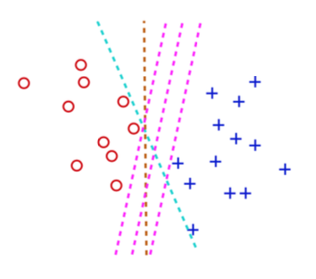
Fig. 84 Draw a line to separate two clusters¶

Suppose there is a hyperplane in \(p\)-dimensional space characterized by the equation

\[ w_{1} x_{1}+w_{2} x_{2}+\cdots+w_{p} x_{p} + b = 0 \]

or in vector form,

\[ \boldsymbol{w} ^\top \boldsymbol{x} + b = 0 \]

Then the distance from any point \(\boldsymbol{x} \in \mathbb{R} ^p\) to this hyperplane can be shown to be

\[ d = \frac{1}{\left\Vert \boldsymbol{w} \right\Vert}\left\vert \boldsymbol{w} ^\top \boldsymbol{x} + b\right\vert \]

Given \(n\) points \(\boldsymbol{x} _1, \ldots, \boldsymbol{x} _n\), for those points in the same side of the hyperplane, they have the same sign of \(\boldsymbol{w} ^\top \boldsymbol{x}_i + b\). If we label the points with positive values of \(\boldsymbol{w} ^\top \boldsymbol{x}_i + b\) by \(y_i = 1\) and those with negative values by \(y_i = -1\), then the distance can be written as

\[ \frac{1}{\left\Vert \boldsymbol{w} \right\Vert } y_i (\boldsymbol{w} ^\top \boldsymbol{x}_i + b ) \]

Definition (Margin): The margin is defined as the shortest distance from a point to the hyperplane.

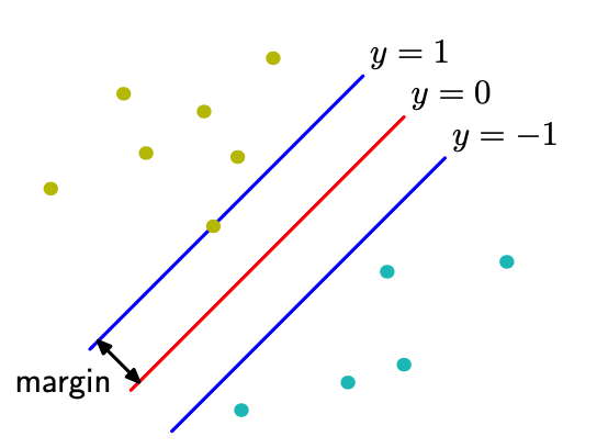
\[ \min _{i} \frac{1}{\left\| \boldsymbol{w} \right\| } y_{i}\left(\boldsymbol{w}^{\top} \boldsymbol{x}_{i}+b\right) \]

Fig. 85 Margin [Bishop]¶

The objective of SVM is to find a hyperplane \(\boldsymbol{w}^{\top} \boldsymbol{x}+b = 0\) parameterized by \(\boldsymbol{w}\) and \(b\), that separates two types of points and maximizes the margin.

\[ \max _{\boldsymbol{w}, b}\left\{\min _i \frac{1}{\|\boldsymbol{w}\|} y_{i}\left(\boldsymbol{w}^{\top} \boldsymbol{x}_{i}+b\right)\right\} \]

i.e.,

\[ \max _{\boldsymbol{w}, b} \frac{1}{\|\boldsymbol{w}\|} \left\{\min _i y_{i}\left(\boldsymbol{w}^{\top} \boldsymbol{x}_{i}+b\right)\right\} \]

To classify a point with coordinates \(\boldsymbol{x}\), we use the solution \(\boldsymbol{w}^*\) and \(b^*\).

If \(\boldsymbol{w}^{* \top} \boldsymbol{x} + b^* > 0\) then \(\hat{y}_i = 1\)
If \(\boldsymbol{w}^{* \top} \boldsymbol{x} + b^* < 0\) then \(\hat{y}_i = -1\)

Learning¶

We convert the optimization problem step by step such that it becomes easier to solve.

Note that distance is invariant to scaling of \(\boldsymbol{w}\) and \(b\) (or note that \(\boldsymbol{w} ^\top \boldsymbol{x} +b = 0\) and \((k\boldsymbol{w}) ^\top \boldsymbol{x} + (kb) = 0\) characterize the same hyperplane), thus we can assume \(\min _{i} y_{i}\left(\boldsymbol{w}^{\top} \boldsymbol{x}_i + b\right)=1\)

Then the maximization-minimization problem becomes a constrained maximization problem

\[\begin{split}\begin{align} \underset{\boldsymbol{w}, b}{\max }&\quad \frac{1}{\|\boldsymbol{w}\|}\\ \text {s.t.}&\quad \min_{i} y_{i}\left(\boldsymbol{w}^{\top} \boldsymbol{x}_i+b\right)=1\\ \end{align}\end{split}\]

Or equivalently,

\[\begin{split}\begin{align} \underset{\boldsymbol{w}, b}{\min }&\quad \frac{1}{2} \boldsymbol{w} ^\top \boldsymbol{w} \\ \text {s.t.}&\quad y_{i}\left(\boldsymbol{w}^{\top} \boldsymbol{x}_i+b\right)\ge1\\ \end{align}\end{split}\]

To get rid of the constraints on \(\boldsymbol{w}\) and \(b\), we use Lagrangian multiplier method. Let

\[ \mathcal{L}(\boldsymbol{w} ,b,\lambda) = \frac{1}{2} \boldsymbol{w} ^\top \boldsymbol{w} + \sum_i ^n \lambda_i (1-y_i(\boldsymbol{w} ^\top \boldsymbol{x}_i + b)) \]

where \(\lambda_i \ge 0\).

Then the problem becomes

\[\begin{split}\begin{align} \underset{\boldsymbol{w}, b}{\min } \, \max _{\boldsymbol{\lambda}} &\quad \mathcal{L}(\boldsymbol{w} ,b, \boldsymbol{\lambda}) \\ \text {s.t.}&\quad \lambda_i \ge 0\\ \end{align}\end{split}\]

Since \(\min_{\boldsymbol{w} ,b} L\) is better to solve than \(\max_{\boldsymbol{\lambda} } L\), we want to exchange the min-max order. This step is valid since it is a quadratic minimization with \(n\) linear constraints, where strong duality holds. As a result, its dual problem is

\[\begin{split}\begin{align} \max _{\boldsymbol{\lambda}} \, \underset{\boldsymbol{w}, b}{\min } &\quad \mathcal{L}(\boldsymbol{w} ,b, \boldsymbol{\lambda}) \\ \text {s.t.}&\quad \lambda_i \ge 0\\ \end{align}\end{split}\]

which is has the same solutions \(\boldsymbol{w}^*, b^*\) with the primal problem.

We first solve the minimization problem. Taking derivatives of \(\mathcal{L}\) w.r.t. \(\boldsymbol{w} ,b\) and equating them to zero gives

\[\begin{split}\begin{align} && \frac{\partial}{\partial \boldsymbol{w}} \mathcal{L} \left(\boldsymbol{w}, b, \boldsymbol{\lambda}\right) &= \boldsymbol{w}-\sum_{i=1}^{n} \lambda_{i} y_{i} \boldsymbol{x}_{i}\overset{\text{set}}{=} 0 \\ &\Rightarrow & \boldsymbol{w} &= \sum_{i=1}^{n} \lambda_{i} y_{i} \boldsymbol{x}_{i} \\ && \frac{\partial}{\partial b} \mathcal{L} \left(\boldsymbol{w}, b, \boldsymbol{\lambda}\right) & =-\sum_{i=1}^{n} \lambda_{i} y_{i} \overset{\text{set}}{=} 0 \\ &\Rightarrow & \sum_{i=1}^{n} \lambda_{i} y_{i} & = 0 \\ \end{align}\end{split}\]

Substituting the result back to the dual problem gives

\[\begin{split}\begin{align} \max _{\boldsymbol{\lambda}} \, &\quad \sum_{i=1}^{n} \lambda_{i}-\frac{1}{2} \sum_{i=1}^{n} \sum_{j=1}^{n}\lambda_{i} \lambda_{j} y_{i} y_{j} \boldsymbol{x}_{i} \boldsymbol{x}_{j} \\ \text {s.t.}&\quad \sum_{i=1}^{n} \lambda_{i} y_{i}=0, \lambda_{i} \geq 0\\ \end{align}\end{split}\]

Solving this quadratic program with linear constraints yields \(\boldsymbol{\lambda} ^*\).

Besides, due to strong duality, KKT conditions hold, such that

\[ \exists\left(x_{k}, y_{n}\right):\, 1-y_{k}\left(\boldsymbol{w} ^{*\top} \boldsymbol{x}_{k}+b\right)=0 \]

which gives \(b^* = y_k - \boldsymbol{w} ^{* \top} \boldsymbol{x} _k\). Therefore,

\[ \boldsymbol{w} ^{*}=\sum_{i=0}^{n} \lambda_{i} y_{i} \boldsymbol{x}_{i} \quad b^{*}=y_{k}-\sum_{i=0}^{n} \lambda_{i} y_{i} \boldsymbol{x}_{i}^{\top} \boldsymbol{x}_{k} \]

Properties¶

The weights is a linear combination of data vectors

\[ \boldsymbol{w} ^{*}=\sum_{i=0}^{n} \lambda_{i} y_{i} \boldsymbol{x}_{i} \]

where \(\lambda_i \ne 0\) for the points that lies on the margin, i.e. only the data on the margin defines \(\boldsymbol{w}^*\).

Moreover,

If \(\boldsymbol{w}^{* \top} \boldsymbol{x} + b^* = \pm 1\) then the point lie on the hyperplane \(\pm\) margin. The vector \(\boldsymbol{x}\) is called a support vector.
If \(\left\vert \boldsymbol{w}^{* \top} \boldsymbol{x} + b^* \right\vert < 1\) then the point lie inside the two margins.
If \(\left\vert \boldsymbol{w}^{* \top} \boldsymbol{x} + b^* \right\vert > 1\) then the point lie outside the two margins.
- If we add more such points to the data set (with correct labels) and re-run SVM, then the solution is the same, since they do not affect \(\min _{i} \frac{1}{|\boldsymbol{w}|} y_{i} \left( \boldsymbol{w} ^ {\top} \boldsymbol{x}_{i}+b\right)\) in the objective function.
maximized margin is

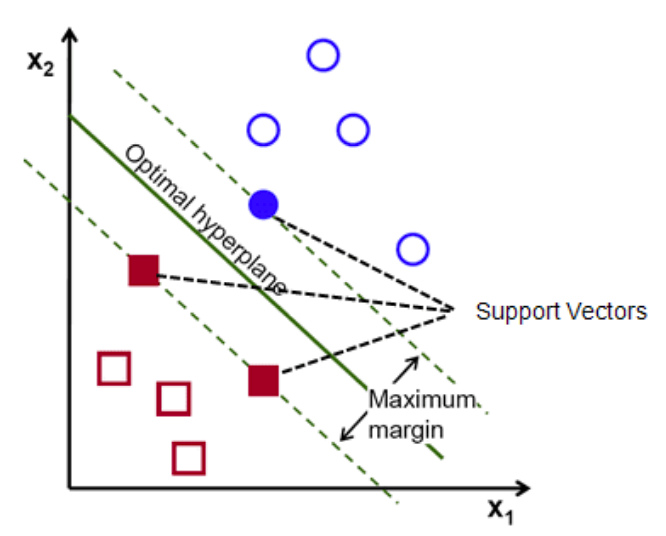
Fig. 86 Support vectors¶

Extension¶

Multiclass¶

One-versus-rest: construct \(K\) separate SVMs. Using \(k^*=\arg \max _{k} (\boldsymbol{w}_k ^\top \boldsymbol{x} + b_k)\)

One-versus-one: construct \(\frac{K(K-1)}{2}\) SVMs on all pairs. Each SVM classifies a point to either \(k_1\) or \(k_2\). For prediction, select \(k\) with the highest votes.

“True” multi-class SVMs (Crammer and Singer, 2001)

Soft Margin¶

Recall the objective function for the hard margin case

\[\begin{split}\begin{aligned} \min _{\boldsymbol{w}, b} &\ \frac{1}{2} \boldsymbol{w}^{\top} \boldsymbol{w} \\ \text { s.t. } &\ y_{i}\left(\boldsymbol{w}^{\top} \boldsymbol{x}_{i}+b\right) \geq 1 \end{aligned}\end{split}\]

What if we cannot find a hyperplane that separate the two types of points? That is, the constraint

\[ y_{i}\left(\boldsymbol{w}^{\top} \boldsymbol{x}_{i}+b\right) \geq 1 \]

does not hold for all \(i\). Some observation will violate this constraint.

In such case, we can add a loss term to measure the extent of violation, and include this loss into the objective function. This kind of margin is called soft margin.

The new objective function becomes

\[ \min _{\boldsymbol{w}, b} \frac{1}{2} \boldsymbol{w}^{\top} \boldsymbol{w} + C\sum_i^n R(\boldsymbol{w} ,b, \boldsymbol{x}_i ,y_i) \]

where

\(R\) is some loss function.
\(C\) is a parameter to control the weight on the loss term. When \(C\rightarrow \infty\), the formulation approaches separable case.

For instance, \(R\) can be an indicator function, with value \(1\) if the constraint is violated, i.e.

\[\begin{split} \begin{equation} R(\boldsymbol{w} ,b, \boldsymbol{x}_i ,y_i) =\left\{\begin{array}{ll} 1, & \text { if } y_{i}\left(\boldsymbol{w}^{\top} \boldsymbol{x}_{i}+b\right) < 1 \\ 0, & \text { otherwise } \end{array}\right. \end{equation} \end{split}\]

A more reasonable loss is to measure the actual deviation from the constrain, i.e., \(1 - y_{i}\left(\boldsymbol{w}^{\top} \boldsymbol{x}_{i}+b\right)\), for those who violates the constraint, i.e. \(y_{i}\left(\boldsymbol{w}^{\top} \boldsymbol{x}_{i}+b\right) < 1\). Overall, the loss function is

\[ R(\boldsymbol{w} ,b, \boldsymbol{x}_i ,y_i) = \max \left\{ 0, 1 - y_{i}\left(\boldsymbol{w}^{\top} \boldsymbol{x}_{i}+b\right) \right\} \]

which is called Hinge loss.

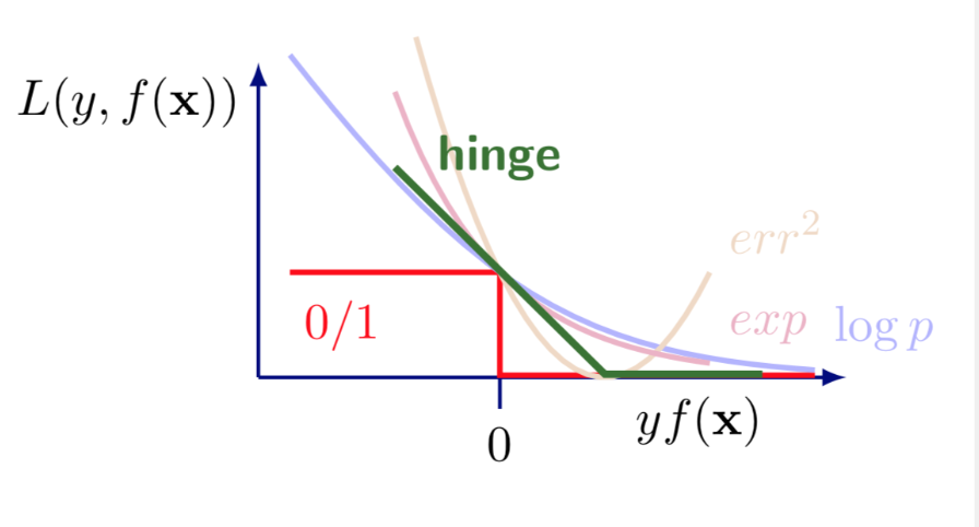
Fig. 87 Comparison of loss functions¶

Let \(\xi_{i}=\max \left\{0,1-y_{i}\left(\boldsymbol{w}^{\top} x_{i}+w_{0}\right)\right\}\), then the objective is

\[ \min _{\boldsymbol{w}, b} \frac{1}{2} \boldsymbol{w}^{\top} \boldsymbol{w} + C\sum_i^n \xi_i \]

From optimization point of view \(\xi_i\) is called a slack variable.

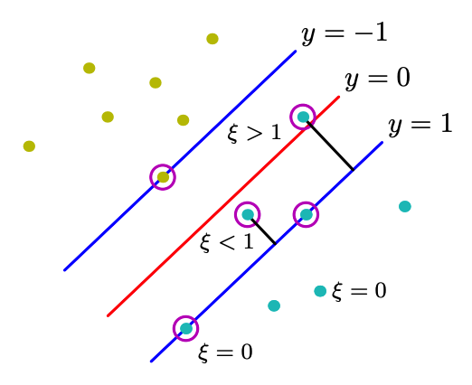
Fig. 88 Hinge loss of data points [Bishop]¶

Applying similar conversion to the basic case above, we get

\[\begin{split}\begin{align} \underset{\boldsymbol{w}, b}{\min }&\quad \sum_{i=1}^{n} \alpha_{i}-\frac{1}{2} \sum_{i, j=1}^{n} \alpha_{i} \alpha_{j} y_{i} y_{j} \boldsymbol{x}_{i} \boldsymbol{x}_{j} \\ \text {s.t.}&\quad \sum_{i=1}^{n} \alpha_{i} y_{i}=0\\ & \quad 0 \leq \alpha_{i} \leq C \end{align}\end{split}\]

This can be solved by gradient descent.

Kernel SVMs¶

If the points are non-seperable, we consider transform them into a higher-dimensional space by a feature transformation \(\boldsymbol{\boldsymbol{\phi}}(\boldsymbol{x})\), and find a hyperplane there to separate the points (hopefully).

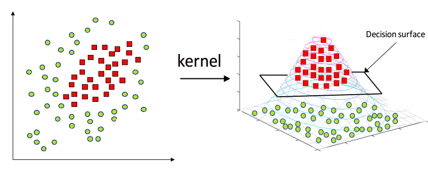
Fig. 89 SVM Kernel trick¶

Transformed Unconstrained Original¶

For the original problem, after transformation into \(\boldsymbol{\phi}(\boldsymbol{x})\) it becomes

\[ \mathcal{L}\left(\boldsymbol{w}, w_{0}\right)=\frac{1}{2}\|\boldsymbol{w}\|^{2}+C \sum_{i=1}^{n} \max \left\{0,1-y_{i}\left(\boldsymbol{w}^{\top} \boldsymbol{\phi}(\boldsymbol{x})+w_{0}\right)\right\} \]

By the Representer Theorem and some refinement, the optimal solution has the form

\[ \boldsymbol{w}^{*}=\sum_{i=1}^{n} \alpha_{i} y_{i} \boldsymbol{\phi}\left(\boldsymbol{x}_{i}\right) \]

Substituting it back to the objective function gives

\[ \|\boldsymbol{w}\|^{2}=\left(\sum_{i=1}^{n} \alpha_{i} y_{i} \boldsymbol{\phi}\left(\boldsymbol{x}_{i}\right)\right)^{\top}\left(\sum_{i=j}^{n} \alpha_{j} y_{j} \boldsymbol{\phi}\left(\boldsymbol{x}_{j}\right)\right)=\sum_{i, j} \alpha_{i} \alpha_{j} y_{i} y_{j} k\left(\boldsymbol{x}_{i}, \boldsymbol{x}_{j}\right) \]

and

\[ \boldsymbol{w}^{\top} \boldsymbol{\phi}(\boldsymbol{x})=\left(\sum_{i=1}^{n} \alpha_{i} y_{i} \boldsymbol{\phi}\left(\boldsymbol{x}_{i}\right)\right)^{\top} \boldsymbol{\phi}(\boldsymbol{x})=\sum_{i} \alpha_{i} y_{i} k\left(\boldsymbol{x}_{i}, \boldsymbol{x}\right) \]

So we turn \(\mathcal{L}\left(\boldsymbol{w}, w_{0}\right)\) to \(\mathcal{L}\left(\boldsymbol{\alpha} , w_{0}\right)\) and we can then solve it by SGD.

Transformed Dual¶

The primal problem becomes

\[\begin{split} \begin{aligned} \underset{\boldsymbol{w}, w_{0}}{\min }&\ \frac{1}{2}\|\boldsymbol{w}\|^{2} \\ \text { s.t.}&\ y_{i}\left(\boldsymbol{w}^{\top} \boldsymbol{\phi}( \boldsymbol{x}_{i}) + w_{0}\right) \geq 1-\xi_{i}, \xi_{i} \geq 0, \forall i \\ &\ \boldsymbol{w}, \boldsymbol{\phi}(\boldsymbol{x}_{i}) \in \mathbb{R}^{d} \end{aligned} \end{split}\]

and the dual problem becomes

\[\begin{split} \begin{aligned} \underset{\boldsymbol{\alpha}}{\max } & \ \left\{\sum_{i=1}^{n} \alpha_{i}-\frac{1}{2} \sum_{i=1}^{n} \sum_{j=1}^{n} \alpha_{i} \alpha_{j} y_{i} y_{j} \boldsymbol{\phi}\left(\boldsymbol{x}_{i}\right)^{\top} \boldsymbol{\phi}\left(\boldsymbol{x}_{j}\right)\right\} \\ \text { s.t.}&\ \sum_{i=1}^{n} \alpha_{i} y_{i}=0,0 \leq \alpha_{i} \leq C, \forall i \end{aligned} \end{split}\]

We find there is a dot product in the objective function, so we can consider using a PSD kernel \(k(\boldsymbol{x} , \boldsymbol{y} )=\boldsymbol{\phi}(\boldsymbol{x} )^{\top} \boldsymbol{\phi}(\boldsymbol{y} )\). The problem becomes

\[\begin{split} \begin{aligned} \underset{\boldsymbol{\alpha}}{ \max }&\ \left\{\sum_{i=1}^{n} \alpha_{i}-\frac{1}{2} \sum_{i=1}^{n} \sum_{j=1}^{n} \alpha_{i} \alpha_{j} y_{i} y_{j} k\left(\boldsymbol{x}_{i}, \boldsymbol{x}_{j}\right)\right\} \\ \text { s.t.} &\ \sum_{i=1}^{n} \alpha_{i} y_{i}=0,0 \leq \alpha_{i} \leq C, \forall i \end{aligned} \end{split}\]

and we solve the QP problem for \(\boldsymbol{\alpha}\).

Pros and Cons¶

Pros

Based on a theoretical model of learning explicitly, with guaranteed performance.
Not affected by local minima.
Do not suffer from the curse of dimensionality.
Quadratic program, doable.
Optimization algorithm instead of greedy search.
Integrated into other high performers such as deep neural networks.
Kernel trick

Cons

Do not directly output probablitity, only scores
- there are some methods to output class membership probability estimates, e.g. Platt scaling, which use logistic regression on the output scores and cross-validation. see here.

Data Science Handbook