.md .pdf

repository open issue

Contents

Linear Discriminant Analysis

We introduce Fisher’s Linear Discriminant Function.

Objective

We have two groups of data in \(\mathbb{R} ^p\)

• \(\left\{ \boldsymbol{x} _{1i} \right\}, i = 1, 2, \ldots, n_1\)

• \(\left\{ \boldsymbol{x} _{2i} \right\}, i = 1, 2, \ldots, n_2\)

We want to project them to a one dimensional line in \(\mathbb{R}\), such that the projection by this line yields good separation of the two classes.

Let the projection be \(\boldsymbol{a} ^{\top} \boldsymbol{x}\) and let the projected data be

• \(\left\{ y _{1i} = \boldsymbol{a} ^{\top} \boldsymbol{x} _{1i} \right\}\)

• \(\left\{ y_{2i} = \boldsymbol{a} ^{\top} \boldsymbol{x} _{2i} \right\}\)

The goodness of separation is measured by th ratio of between-class difference and within-class variance.

\[ \max _ {\boldsymbol{a} \in \mathbb{R} ^p} \frac{(\bar{y}_1- \bar{y}_2)^2}{s_y^2} \]

where \(s_y^2\) is the pooled variance, if we assume equal covariance structure in the two groups.

\[ s_{y}^{2}=\frac{\sum_{i=1}^{n_{1}}\left(y_{1 i}-\bar{y}_{1}\right)^{2}+\sum_{i=1}^{n_{2}}\left(y_{2 i}-\bar{y}_{2}\right)^{2}}{n_{1}+n_{2}-2}=\boldsymbol{a} ^{\top} \boldsymbol{S}_{x} \boldsymbol{a}=\boldsymbol{a}^{\top} \boldsymbol{S}_{\text {pool }} \boldsymbol{a} \]

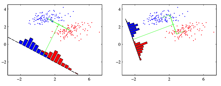
Fig. 83 Illustration of projection of data to a linear direction [C. Bishop, 2006]

Assumptions

• equal covariance matrix \(\boldsymbol{\Sigma} _1 = \boldsymbol{\Sigma} _2 = \boldsymbol{\Sigma}\)

• full rank \(\operatorname{rank}\left( \boldsymbol{\Sigma} \right) = p\)

• without normality assumption that the population are from multivariate normal.

Learning

Note that the objective function

\[ \frac{(\bar{y}_1- \bar{y}_2)^2}{s_y^2} = \frac{[\boldsymbol{a} ^{\top} (\bar{\boldsymbol{x} }_1-\bar{\boldsymbol{x} }_2)]^2}{\boldsymbol{a}^{\top} \boldsymbol{S}_{\text {pool }} \boldsymbol{a}} \]

has the form of generalized Rayleigh quotient. Hence the solution is given by

\[ \boldsymbol{a} ^*= \boldsymbol{S} _{\text{pool} } ^{-1} (\bar{\boldsymbol{x} }_1-\bar{\boldsymbol{x} }_2) \]

with maximum

\[ (\bar{\boldsymbol{x} }_1-\bar{\boldsymbol{x} }_2) \boldsymbol{S} _{\text{pool} } ^{-1} (\bar{\boldsymbol{x} }_1-\bar{\boldsymbol{x} }_2) =: D^2 \]

The maximum \(D^2\) can be viewed as the square of the Mahalanobis distance between the population means of the original data.

Prediction

For a new data point \(\boldsymbol{x} _0\), we compute \(y_0 = \boldsymbol{a} ^{* \top } \boldsymbol{x} _0\), and see whether \(y_0\) is closer to \(\bar{y}_1\) or \(\bar{y}_2\). Below are two equivalent classification rules.

• Define the midpoint of the transformed means \(m = \frac{1}{2}(\bar{y}_1 + \bar{y}_2)\) as the partition point, suppose \(\bar{y}_1 \ge \bar{y}_2\), then

  \[ R_1: \quad y_0 \ge \frac{1}{2}(\bar{y}_1 + \bar{y}_2) \]

• Assign it to closer class, in terms of absolute distance

  \[j^* = \min_{j=1, 2} \left\vert y_0 - \bar{y}_j \right\vert\]

• Assign it to closer class, in terms of squared distance

  \[ R_1: \quad (y_0 - \bar{y}_1)^2 \le (y_0 - \bar{y}_2)^2 \]

  or using \(\boldsymbol{x}\)

  \[ R_1: \quad \left\vert \boldsymbol{a} ^{* \top} (\boldsymbol{x} _0 - \bar{\boldsymbol{x} }_1) \right\vert^2 \le \left\vert \boldsymbol{a} ^{* \top} (\boldsymbol{x} _0 - \bar{\boldsymbol{x} }_2) \right\vert^2 \]

Related to

Two-sample Means

The quantity \(D^2\) is used in Hotelling’s \(T^2\) to test if the two means are equal. The test can be used here to check if the separation of the two population is significant enough to apply classification. Under the assumption of normal distribution of equal variance for the two populations, the test statistic is

\[ \frac{n_{1}+n_{2}-p-1}{\left(n_{1}+n_{2}-2\right) p} \cdot \frac{n_{1} n_{2}}{n_{1}+n_{2}} D^{2} \sim F_{p, n_{1}+n_{2}-p-1} \quad \text { under } \quad H_{0}: \boldsymbol{\mu}_{1}=\boldsymbol{\mu}_{2} \]

There is not much point to conduct classification if the difference of the class means is not significant in the first place. On the other hand, significant difference of the class means is not sufficient to guarantee a good classification.

Discriminant for Gaussian Data

Recall that for two Gaussian population, under the assumptions on equal covariance, equal costs and equal prior, the sample linear classification function that minimizes ECM is

\[ \left(\bar{\boldsymbol{x} }_{1}-\bar{\boldsymbol{x} }_{2}\right)^{\top} \boldsymbol{S} _{\text{pool} }^{-1} {\color{teal}{\boldsymbol{x}_{0}}} \ge\frac{1}{2}\left(\bar{\boldsymbol{x} }_{1}-\bar{\boldsymbol{x} }_{2}\right)^{\top} \boldsymbol{S} _{\text{pool} }^{-1}\left(\bar{\boldsymbol{x} }_{1}+\bar{\boldsymbol{x} }_{2}\right) \]

Substituting \(\boldsymbol{a} ^{* \top} = \left(\bar{\boldsymbol{x} }_{1}-\bar{\boldsymbol{x} }_{2}\right)^{\top} \boldsymbol{S} _{\text{pool} }^{-1}\) gives

\[ \boldsymbol{a} ^{\top} {\color{teal}{\boldsymbol{x}_{0}}} \ge \frac{1}{2} \boldsymbol{a} ^{\top}\left(\bar{\boldsymbol{x} }_{1}+\bar{\boldsymbol{x} }_{2}\right) \]

which is exactly the Fisher LDA classification rule \(y_0 \ge m\). Hence, Fisher arrived at same conclusions from a different perspective, without the normal assumption, which also testifies the ubiquitous nature of normal distributions.

Multi-classes

We can extend two classes to multi-classes, and extend projection to one line to projection to some dimensions, i.e. as a dimensionality reduction method.

The assumptions remain the same

• equal covariance matrix \(\boldsymbol{\Sigma} _1 = \ldots = \boldsymbol{\Sigma} _g = \boldsymbol{\Sigma}\)

• full rank \(\operatorname{rank}\left( \boldsymbol{\Sigma} \right) = p\)

• without normality assumption that the population are from multivariate normal.

Learning

We first consider projection to one line case. The objective is to maximize

\[ \frac{\boldsymbol{a} ^{\top}\{\text { between group variance matrix }\} \boldsymbol{a} }{\boldsymbol{a} ^{\top}\{\text { within group variance matrix }\} \boldsymbol{a} }=\frac{\boldsymbol{a} ^{\top} \boldsymbol{B} \boldsymbol{a} }{\boldsymbol{a} ^{\top} \boldsymbol{W} \boldsymbol{a} } \]

where

• between-group variance matrix (different from \(\boldsymbol{B}\) in MANOVA)

  \[\boldsymbol{B}=\sum_{i=1}^{g}\left(\bar{\boldsymbol{x}}_{i}-\bar{\boldsymbol{x}}\right)\left(\bar{\boldsymbol{x}}_{i}-\bar{\boldsymbol{x}}\right)^{\top}\]

• mean-of-means, aka overall average, in contrast to grand average

  \[\bar{\boldsymbol{x}} = \frac{1}{g} \sum_{i=1}^g \bar{\boldsymbol{x}}_i\]

• within-group variance matrix (same \(\boldsymbol{W}\) in MANOVA)

  \[\boldsymbol{W}=\sum_{i=1}^{g}\left(n_{i}-1\right) \boldsymbol{S}_{i}=\sum_{i=1}^{g} \sum_{j=1}^{n_{i}}\left(\boldsymbol{x}_{i j}-\bar{\boldsymbol{x}}_{i}\right)\left(\boldsymbol{x}_{i j}-\bar{\boldsymbol{x}}_{i}\right)^{\top}\]

This is again a generalized Rayleigh quotient. The optimizer \(\boldsymbol{a} ^*\) and maximum is given by the largest eigen pair of matrix \(\boldsymbol{W} ^{-1} \boldsymbol{B}\).

\[ \boldsymbol{W} ^{-1} \boldsymbol{B} \boldsymbol{a} ^*= \lambda \boldsymbol{a}^* \]

Recall that \(\boldsymbol{S} _{\text{pool} } = \frac{1}{n-g} \boldsymbol{W}\). The eigenvector \(\boldsymbol{a} ^*\) is usually chosen such that

\[ \boldsymbol{a} ^{* \top} \boldsymbol{S} _{\text{pool} } \boldsymbol{a} ^*=1 \]

After obtain one projection direction \(\boldsymbol{a} _1 ^*\), we can continue for next, i.e. second largest eigenvector, and so on. There eigenvectors \(\boldsymbol{a} _j ^*\) are called discriminant coordinates, or canonical variates, coming from an alternative derivation via CCA on predictor variable matrix and response variable matrix.

Note that there are at most \(r\) non-zero eigenvalues of \(\boldsymbol{W} ^{-1} \boldsymbol{B}\) where

\[ r=\operatorname{rank}\left(\boldsymbol{W}^{-1} \boldsymbol{B}\right) \leq \min (g-1, p) \]

Therefore the above method can produce up to \(r\) linear discriminants.

By the maximum procedure and proper scaling, we have

\[\begin{split}\boldsymbol{a} _{i} ^{* \top} \boldsymbol{S} _{\text{pool} } \boldsymbol{a} ^*_{j}=\left\{\begin{array}{ll} 1 & \text { if } i=j \leq r \\ 0 & \text { otherwise } \end{array}\right.\end{split}\]

Interpretation

They give consecutive directions that maximized the normalized variance between classes, they are not discriminant function themselves. Analogous to the principal components in PCA, hopefully the first few sample discriminants show better separation of the groups, and can be used to classify new observations.

Prediction

Recall that for \(g=2\) case, the classification rule using squared distance is

\[ R_1: \quad \left\vert \boldsymbol{a} ^{\top} (\boldsymbol{x} _0 - \bar{\boldsymbol{x} }_1) \right\vert^2 \le \left\vert \boldsymbol{a} ^{\top} (\boldsymbol{x} _0 - \bar{\boldsymbol{x} }_2) \right\vert^2 \]

In case of \(r\) discriminant coordinates \(\boldsymbol{a} _1, \ldots, \boldsymbol{a} _r\), we allocate \(\boldsymbol{x} _0\) to class \(k\) if

\[ \sum_{i=1}^{r}\left|\boldsymbol{a} _{i}^{\top}\left(\boldsymbol{x} _{0}-\bar{\boldsymbol{x} }_{k}\right)\right|^{2} \leq \sum_{i=1}^{r}\left|\boldsymbol{a} _{i}^{\top}\left(\boldsymbol{x} _{0}-\bar{\boldsymbol{x} }_{j}\right)\right|^{2}, \quad \text { for any } j=1, \cdots, g \]

Equivalently,

\[ \left\| \boldsymbol{A} ^{\top} (\boldsymbol{x} _0 - \boldsymbol{x} _k) \right\|^2 \leq \left\| \boldsymbol{A} ^{\top} (\boldsymbol{x} _0 - \boldsymbol{x} _j) \right\|^2, \quad \text { for any } j=1, \cdots, g \]

where \(\boldsymbol{A} \in \mathbb{R} ^{p \times r}\) and consists \(r\) scaled eigenvectors such that \(\boldsymbol{A} ^{\top} \boldsymbol{S} _{\text{pool} }\boldsymbol{A} = \boldsymbol{I} _r\).

R.t. Discriminant for Gaussian Data

In the \(g=2\) case above, we showed that Fisher LDA is equivalent to the linear discriminant rule for Gaussian that minimizes ECM under some assumptions. Now we show they are equivalent in \(g \ge 2\) case, under those assumptions.

Recall that under the assumptions on equal covariance, equal costs, and equal priors, the sample classification rule for multi-classes that minimizes ECM is

\[\begin{split}\begin{aligned} R_{k} &=\left\{\boldsymbol{x}: \hat{d}_{k}(\boldsymbol{x}) \geq \hat{d}_{i}(\boldsymbol{x}), \text { for all } i \neq k\right\} \\ &=\left\{\boldsymbol{x}: \hat{d}_{k}(\boldsymbol{x})=\max \left\{\hat{d}_{1}(\boldsymbol{x}), \cdots, \hat{d}_{g}(\boldsymbol{x})\right\}\right\} \end{aligned}\end{split}\]

where

\[ \hat{d}_{k}(\boldsymbol{x})=\bar{\boldsymbol{x}}_{k}^{\top} \boldsymbol{S} _{\text {pool }}^{-1} \boldsymbol{x}-\frac{1}{2} \bar{\boldsymbol{x}}_{k}^{\top} \boldsymbol{S} _{\text {pool }}^{-1} \bar{\boldsymbol{x}}_{k} \]

In Fisher LDA, assume \(r = p\), let the eigenvector matrix be \(\boldsymbol{A}_{p \times p} = [\boldsymbol{a} _1, \boldsymbol{a} _2, \ldots, \boldsymbol{a} _p]\), then we have

\[\begin{split}\begin{aligned} \boldsymbol{A} ^{\top} \boldsymbol{S} _{\text{pool} }\boldsymbol{A} &= \boldsymbol{I} _p \\ \Rightarrow \qquad \boldsymbol{S} _{\text{pool} } &= \boldsymbol{A} ^{-\top} \boldsymbol{A} ^{-1} \\ \Rightarrow \qquad \boldsymbol{S} _{\text{pool} } ^{-1} &= \boldsymbol{A} \boldsymbol{A} ^{\top} \\ \end{aligned}\end{split}\]

In the Fisher LDA classification rule, the distance can be written as

\[\begin{split}\begin{aligned} \sum_{i=1}^{r}\left|\boldsymbol{a} _{i}^{\top}\left(\boldsymbol{x} _{0}-\bar{\boldsymbol{x} }_{k}\right)\right|^{2} &= \left\| \boldsymbol{A} ^{\top} (\boldsymbol{x} _0 - \bar{\boldsymbol{x} }_k) \right\| _2^2 \\ &= (\boldsymbol{x} _0 - \bar{\boldsymbol{x} }_k) ^{\top} \boldsymbol{A} \boldsymbol{A} ^{\top} (\boldsymbol{x} _0 - \bar{\boldsymbol{x} }_k)\\ &= (\boldsymbol{x} _0 - \bar{\boldsymbol{x} }_k) ^{\top} \boldsymbol{S} _{\text{pool} } ^{-1} (\boldsymbol{x} _0 - \bar{\boldsymbol{x} }_k)\\ &= \boldsymbol{x} _0 ^{\top} \boldsymbol{S} _{\text{pool} } ^{-1}\boldsymbol{x} _0 - 2 \bar{\boldsymbol{x} }_k \boldsymbol{S} _{\text{pool} } ^{-1} \boldsymbol{x} _0 + \bar{\boldsymbol{x} }_k \boldsymbol{S} _{\text{pool} } ^{-1}\bar{\boldsymbol{x} }_k\\ \end{aligned}\end{split}\]

Therefore, the Fisher LDA classification rule is

\[\begin{split}\begin{aligned} k^* &= \arg \min _k\ \sum_{i=1}^{r}\left|\boldsymbol{a} _{i}^{\top}\left(\boldsymbol{x} _{0}-\bar{\boldsymbol{x} }_{k}\right)\right|^{2} \\ &= \arg \min _k\ - 2 \bar{\boldsymbol{x} }_k \boldsymbol{S} _{\text{pool} } ^{-1} \boldsymbol{x} _0 + \bar{\boldsymbol{x} }_k \boldsymbol{S} _{\text{pool} } ^{-1}\bar{\boldsymbol{x} }_k \\ &= \arg \max _k\ \bar{\boldsymbol{x} }_k \boldsymbol{S} _{\text{pool} } ^{-1} \boldsymbol{x} _0 - \frac{1}{2} \bar{\boldsymbol{x} }_k \boldsymbol{S} _{\text{pool} } ^{-1}\bar{\boldsymbol{x} }_k \\ &= \arg \max _k\ \bar{\boldsymbol{x} }_k \hat{d}_{k}(\boldsymbol{x})\\ \end{aligned}\end{split}\]

which is exactly the linear classification rule for Gaussian Data, under those assumptions.

previous

For Gaussian Data

next

Support Vector Machine