Large Sample Theory
Convergence in Probability
- Definition (Convergence in probability)
A sequence \({X_n}\) of random variables converges in probability towards the random variable \(X\) if for all \(\varepsilon > 0\),
\[ \lim _{n \rightarrow \infty} \operatorname{\mathbb{P}}\left(\left|X_{n}-X\right|>\varepsilon\right)=0 \]
In short, we write \(X_{n} \stackrel{\mathcal{P}}{\rightarrow} X\) or \(\operatorname{plim} X_{n}=X\).
Properties
\(\operatorname{plim} \frac{X_n}{Y_n} = \frac{\operatorname{plim} X_n }{\operatorname{plim} Y_n }\)
\(\operatorname{plim} X_nY_n = \operatorname{plim} X_n \operatorname{plim} Y_n\)
\(\operatorname{plim} (X_n+Y_n) = \operatorname{plim} X_n + \operatorname{plim} Y_n\)
\(\operatorname{plim} g(X_n) = g(\operatorname{plim} X_n )\) if \(g\) if is continuous at \(\operatorname{plim} X_n\)
Law of Large Numbers
The Law of Large Numbers states that, as the number of identically distributed, randomly generated variables increases, their sample mean (average) approaches their theoretical mean.
Weak Law of Large Numbers
Let \(X_1, \ldots, X_n\) be independently and identically distributed random variables with mean \(\mu\) and variance \(\sigma^{2}<\infty\). Then for every \(\epsilon>0\),
i.e. the sample mean converge in probability to the theoretical mean \(\mu\),
It leaves open the possibility that \(\left|\overline{X}_{n}-\mu \right|>\epsilon\) happens an infinite number of times,
To prove it, by Chebychev’s Inequality,
Strong Law of Large Numbers
Let \(X_1, \ldots, X_n\) be independently and identically distributed random variables with mean \(\mu\) and variance \(\sigma^{2}<\infty\). Then for every \(\epsilon>0\),
i.e. the sample mean converge to the theoretical mean \(\mu\) almost surely,
Note
Converge almost surely is a stronger condition than converge in probability.
In some cases, the strong law does not hold, but the weak law does.
Central Limit Theorem
The Central Limit Theorem, in probability theory, when independent random variables are added, their properly normalized sum tends toward a normal distribution (informally a “bell curve”) even if the original variables themselves are not normally distributed.
There are many versions of CLT with various problem settings. Here we introduce Lindeberg–Lévy CLT.
Let \(X_1, \ldots, X_n\) be a sequence of independently and identically distributed random variables such that \(\operatorname{\mathbb{E}}\left( X_{i} \right)=\mu\), \(\mathrm{Var}\left( X_{i} \right)=\sigma^{2}>0\). Let \(G_{n}(x)\) denote the CDF of \(\frac{\sqrt{n}\left(\bar{X}_{n}-\mu\right)}{\sigma}\), then
i.e., the normalized sample mean converge in distribution to a standard normal random variable,
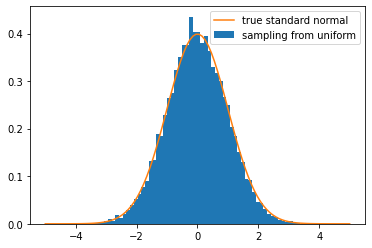
The Central Limit Theorem implies that we can obtain a normal distribution from a uniform random variable generator. Let \(X\sim \mathcal{U}(0,1)\), then \(\mu = \operatorname{\mathbb{E}}\left( X \right) =\frac{1}{2}\), \(\sigma = \sqrt{\mathrm{Var}\left(X \right)} = \sqrt{\frac{1}{12}}\). Hence,
Implementation with Python:
import numpy as np
import matplotlib.pyplot as plt
from scipy.stats import norm

n = 10000 # sample size
m = 10000 # number of samples
means = np.random.rand(m, n).mean(axis=1)
std_means = np.sqrt(n) * (means - 0.5) / np.sqrt(1/12)

points = np.linspace(-5, 5, 100)
true = norm.pdf(points)

plt.hist(std_means, bins='auto', density=True, label='sampling from uniform')
plt.plot(points, true, label='true standard normal')
plt.legend()
plt.show()
In general, one can then sample from any normal distribution \(\mathcal{N}(a,b^2)\) by the transformation \(Z = bY_n+a\).
In multivariate case, when \(n-p\) is large, approximately,
Eigen Analysis of Covariance Matrix
Assume that \(\boldsymbol{x}_i \overset{\text{iid}}{\sim}\mathcal{N} _p(\boldsymbol{\mu} , \boldsymbol{\Sigma} )\), let \((\lambda_i, \boldsymbol{u} _i)\) and \((\hat{\lambda}_i, \hat{\boldsymbol{u}} _i)\) be respectively the eigen pair of population covariance matrix \(\boldsymbol{\Sigma}\) and of sample covariance matrix \(\boldsymbol{S}\). Let \(d_i = \sqrt{n-1} (\hat{\lambda}_i - \lambda_i)\) be a difference measure between the two eigenvalues, and \(\boldsymbol{z} _i = \sqrt{n-1}(\hat{\boldsymbol{u}} _i - \boldsymbol{u} _i)\) be a difference measure between the two eigenvectors, then we have the following asymptotic results as \((n - 1 - p) \rightarrow \infty\),
\([d_1, \ldots, d_p]\) is independent of \([\boldsymbol{z} _1, \ldots, \boldsymbol{z} _p]\)
\(d_i\)’s are independently \(\mathcal{N} (0, 2\lambda_i^2)\).
\(\boldsymbol{z} _i \sim \mathcal{N} _p(\boldsymbol{0} , \sum_{k=1 \atop k \neq i}^{p} \frac{\lambda_{i} \lambda_{k}}{\left(\lambda_{i}-\lambda_{k}\right)^{2}} \boldsymbol{u}_{k} \boldsymbol{u}_{k}^{\top})\) and \(\operatorname{Cov}\left(\boldsymbol{z}_{i}, \boldsymbol{z}_{j}\right)=-\frac{\lambda_{i} \lambda_{j}}{\left(\lambda_{i}-\lambda_{j}\right)^{2}} \boldsymbol{u}_{j} \boldsymbol{u}_{i}^{\top}\)
Inequalities
Chernoff Bound
Chernoff bound gives bounds of the sum of \(n\) random variables over \([0,1]\) (not necessarily independent).
Suppose \(X_{1}, \cdots, X_{n}\) are independent random variables with \(X_{i} \in[0,1]\). Let \(S=\sum_{i} X_{i}\) and \(\mu=\mathbb{E}[S]\) be the expected sum. Then for \(\lambda \in (0,1)\),
and,
Together:
Bernstein Inequality
Univariate Case
Let \(X_1, X_2, \ldots, X_n \in \mathbb{R}\) be i.i.d. random variables with mean 0 and value \(\left\vert X_i \right\vert \le L\). Let their sum be \(S = \sum_{i=1}^n X_i\). Then
If \(n\) is large, since \(\operatorname{Var}\left( S \right) = n \sigma^2\), the bound becomes
Let \(t = \sqrt{n \log n} \cdot \sigma\), then we have
In other words, w.h.p., we have \(\frac{1}{n} \left\vert S \right\vert \le \sqrt{\frac{\log n}{n}} \sigma\).
The term \(Lt/3\) takes into account that each r.v. could be non-Gaussian like.
Random Matrices Case
Let \(\boldsymbol{X}_1, \boldsymbol{X}_2, \ldots, \boldsymbol{X}_n \in \mathbb{R} ^ {d_1 \times d_2}\) be i.i.d. random matrices with mean 0 and spectral norm \(\left\| \boldsymbol{X} _i \right\| \le L\). Let their sum be \(\boldsymbol{S} = \sum_{i=1}^n \boldsymbol{X}_i\) and define the ‘variance’ as
Then
Hoeffding’s Inequality
Let \(Z_i, \ldots, Z_n\) be independent bounded random variables with \(Z_i \in [a, b]\) for all \(i\). Then
and
for all \(t\).