Vector Spaces
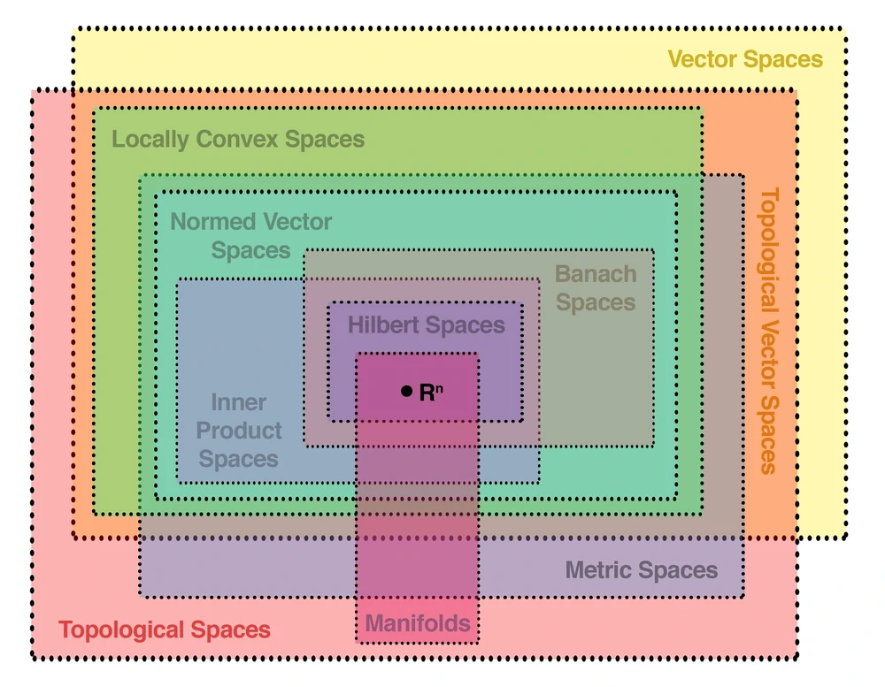
Fig. 1 Venn diagram of vector spaces and other spaces
Vector Spaces
Before defining vector spaces, we first define fields.
Fields
- Definition (Fields)
A field is a set \(F\) with addition and multiplication (mappings \(F\times F \rightarrow F\)), which satisfies all the following axioms
Commutativity: \(\forall a, b \in F, a+b=b+a, a \cdot b=b \cdot a\)
Association: \(\forall a, b, c \in F, (a+b)+c=a+(b+c),(a \cdot b) \cdot c=a \cdot(b \cdot c)\)
Additive and multiplicative identity: \(\exists 0,1 \in F \text { s.t. } \forall a \in F, a+0=a \text { and } a \cdot 1=a\)
Additive inverse: \(\forall a \in F, \exists(-a) \in F, \text { s.t. } a+(-a)=0\)
Multiplicative inverse: \(\forall a \in F(a \neq 0), \exists a^{-1} \in F, \text { s.t. } a \cdot a^{-1}=1\)
Distributivity of multiplication over addition: \(\forall a, b, c \in F, a \cdot(b+c)=a \cdot b+a \cdot c\)
- Examples
\(\mathbb{Q}, \mathbb{R}, \mathbb{C}, \mathbb{F}_{2}, \mathbb{F}_{p}\) (\(p\) is a prime).
Definition
A vector space is defined per field.
- Definition (Vector spaces)
A vector space over field \(F\) is a set \(V\) associated with operations addition and scalar multiplication that satisfies all the following axioms
Association of addition: \(\forall \boldsymbol{u}, \boldsymbol{v}, \boldsymbol{w} \in V,(\boldsymbol{u}+\boldsymbol{v})+\boldsymbol{w}=\boldsymbol{u}+(\boldsymbol{v}+\boldsymbol{w})\)
Commutativity of addition: \(\forall \boldsymbol{u}, \boldsymbol{v} \in V, \boldsymbol{u}+\boldsymbol{v}=\boldsymbol{v}+\boldsymbol{u}\)
Identity element of addition: \(\exists \boldsymbol{0} \in V\) s.t. \(\forall \boldsymbol{v} \in V, \boldsymbol{v}+\boldsymbol{0}=\boldsymbol{v}\)
Compatibility of scalar multiplication with field multiplication: \(\forall a, b \in F, \boldsymbol{v} \in V, a(b \boldsymbol{v})=(a b) \boldsymbol{v}\)
Identity element of scalar multiplication: \(1 \boldsymbol{v}=\boldsymbol{v}\) where \(1\) is the multiplicative identity in \(F\)
Distributivity of scalar multiplication with respect to vector addition: \(\forall a \in F, \boldsymbol{u}, \boldsymbol{v} \in V, a(\boldsymbol{u}+\boldsymbol{v})=a \boldsymbol{u}+a \boldsymbol{v}\)
Distributivity of scalar multiplication with respect to field addition: \(\forall a, b \in F, \boldsymbol{v} \in V,(a+b) \boldsymbol{v}=a \boldsymbol{v}+b \boldsymbol{v}\)
- Examples
\(\mathbb{R}^d\) is a vector space over field \(\mathbb{R}\)
\(\mathbb{R}\) is a vector space over \(\mathbb{Q}\)
All Fibonacci sequences form a vector space over \(\mathbb{R}\)
\[ \left\{\left(x_{1}, x_{2}, x_{3} \ldots\right) \in \mathbb{R}^{\infty} \mid \forall i \geq 1: x_{i}+x_{i+1}=x_{i+2}\right\} \]
Metric Spaces
Definition
- Definition (Metric spaces)
A metric space is an ordered pair \((M, d)\) where \(M\) is a set and \(d\) is a metric function \(d: M \times M \rightarrow \mathbb{R}\) that satisfies all the following axioms
Identity of indiscernibles: \(d(x, y)=0 \Leftrightarrow x= y\)
Symmetry: \(d(x,y) = d(y, x)\)
Triangle inequality: \(d(x, z) \le d(x, y) + d(y, z)\)
Given the above three axioms, we have \(d(x, y) \ge 0\) for any \(x, y \in M\).
The function \(d\) is also called distance function or simply distance. Often, \(d\) is omitted and one just writes \(M\) for a metric space if it is clear from the context what metric is used.
- Examples:
Discrete metric \(d(x,y)=1\) if \(x\ne y\) and \(0\) otherwise.
\(\mathbb{R}\) with absolute difference \(d(x,y) = \left\vert x-y \right\vert\)
\(\mathbb{R} ^n\) with Euclidean distance
\(\mathbb{R} _{>0}\) with \(d(x, y) = \left\vert \log(y/x) \right\vert\)
In practice and in real life, all sensible dissimilarity measures fulfill 2, mostly 1. However it is not so uncommon that a dissimilarity measure fails to satisfy 3.
If correlation \(\rho(\boldsymbol{x}, \boldsymbol{y})\) is used for similarity measure, then \(d(\boldsymbol{x}, \boldsymbol{y}) = \sqrt{2(1-\rho)}\) satisfies 2, 3 but not the \(\Leftarrow\) part of 1. Such measure is called a pseudo-metric.
Completeness
We first introduce Cauchy sequence.
- Definition (Cauchy sequence)
Cauchy sequence is a sequence whose elements become arbitrarily “close” to each other as the sequence progresses. The elements can be in \(\mathbb{R}\) or other spaces. The definition of “close” depends on some metric function.
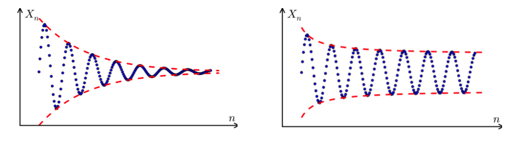
For instance, in \(\mathbb{R}\), \(x_1, x_2, \ldots,\) is called a Cauchy sequence if for every positive number \(\epsilon\), there is a positive integer \(N\) such that for all natural numbers \(m, n>N\),
Pictorially,
- Examples
For any real number \(r\), the sequence of truncated decimal expansions of \(r\) forms a Cauchy sequence. For example, when \(r = \pi\), this sequence is \((3, 3.1, 3.14, 3.141, ...)\). The \(m\)-th and \(n\)-th terms differ by at most \(10^{1-m}\) when \(m < n\), and as \(m\) grows, this becomes smaller than any fixed positive number \(\epsilon\).
- Non-examples
\(x_n = \sqrt{n}\), though each term becomes arbitrarily close to the preceding term
- Definition (Complete metric space)
A metric space \(M\) is called complete if every Cauchy sequence of points in \(M\) has a limit that is also in \(M\), or alternatively, if every Cauchy sequence in \(M\) converges in \(M\) (converges to some point of \(M\)).
- Examples
\(\mathbb{R}\)
- Non-examples
open interval \(A=(0,1)\) with an ordinary distance in \(\mathbb{R}\) is not a complete space: there is a sequence \(x_n = \frac{1}{n}\), which is Cauchy, but does not converge in \(X\), i.e. its limit \(0 \notin A\).
Normed Vector Spaces
- Definition (Normed vector spaces)
A normed vector space or normed space is a vector space \(V\) over the real or complex numbers, on which a norm \(\left\| \cdot \right\|\) is defined, together denoted as \((V, \left\| \cdot \right\| )\).
- Definition (Norm)
A norm is a real-valued function from a real or complex vector space \(V\) to the non-negative real numbers, denoted \(\left\| \cdot \right\| : V \rightarrow \mathbb{R}_{\ge 0}\), that satisfies the following axioms
Positive definite: \(\|x\|=0 \Longleftrightarrow x=0\)
Absolutely homogeneous: \(\|\alpha x\|=|\alpha\|\| x|\)
Triangle inequality: \(\|x+y\| \leq\|x\|+\|y\|\)
A norm is the formalization and the generalization to real vector spaces of the intuitive notion of “length” in the real world.
- Examples
absolute value \(\left\| x \right\| = \left\vert x \right\vert\)
Euclidean norm \(\|\boldsymbol{x}\|_{2}:=\sqrt{x_{1}^{2}+\cdots+x_{n}^{2}}\)
Manhattan norm
Maximum norm
- Relations
Once a norm is defined, we can immediately define a distance by
\[ d(x, y) = \left\| x - y \right\| \]which is called the induced distance by the norm. Hence, any normed vector space is a metric space and a topological vector space.
If the induced distance \(d\) is complete, then the normed vector space is a Banach space
Inner Product Spaces
Aka Hausdorff pre-Hilbert spaces.
- Definition (Inner product spaces)
An inner product space is a vector space \(V\) over a field \(F\) together with a binary operation \(\langle \cdot, \cdot \rangle\) called an inner product.
- Definition (Inner products)
An inner product is a binary operation \(\langle\cdot, \cdot\rangle: V \times V \rightarrow \mathbb{F}\) that satisfies all the following axioms
Linearity in the first argument
\[\begin{split}\begin{aligned} \langle a \boldsymbol{x}, \boldsymbol{y}\rangle &=a\langle\boldsymbol{x}, \boldsymbol{y}\rangle \\ \left\langle\boldsymbol{x}_{1}, \boldsymbol{y}\right\rangle+\left\langle\boldsymbol{x}_{2}, \boldsymbol{y}\right\rangle &=\left\langle\boldsymbol{x}_{1}+\boldsymbol{x}_{2}, \boldsymbol{y}\right\rangle \end{aligned}\end{split}\]Conjugate symmetry (Hermitian symmetry):
\[\langle\boldsymbol{x}, \boldsymbol{y}\rangle=\overline{\langle\boldsymbol{y}, \boldsymbol{x}\rangle}\]Positive definite
\[\begin{split} \langle\boldsymbol{x}, \boldsymbol{x}\rangle \left\{\begin{array}{ll} >0, & \text { if } \boldsymbol{x} \neq \boldsymbol{0} \\ = 0, & \text { otherwise } \end{array}\right. \end{split}\]Note that \(2\) and \(3\) together imply that \(\langle\boldsymbol{x}, \boldsymbol{x}\rangle \in \mathbb{R}_{\geq 0}\).
Inner products associate each pair of vectors in the space with a scalar quantity. They allow the rigorous introduction of intuitive geometrical notions, such as the length of a vector or the angle between two vectors. They also provide the means of defining orthogonality between vectors (zero inner product)
- Examples
standard multiplication over the real numbers: \(\langle x, y \rangle = xy\)
dot product over \(\mathbb{R} ^n\): \(\langle \boldsymbol{x} , \boldsymbol{y} \rangle= \boldsymbol{x} ^{\top} \boldsymbol{y} = \sum_{i=1}^n x_i y_i\)
- Relations
An inner product naturally induces an associated norm \(\left\| x \right\|= \sqrt{ \langle x, x \rangle}\), which canonically makes every inner product space into a normed vector space.
If this normed space is also a Banach space then the inner product space is called a Hilbert space.
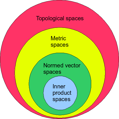
The relations between metric spaces, normed vector spaces and inner product spaces can then be summarized as below:
Hilbert Spaces
Definition
A Hilbert space extends the methods of vector algebra and calculus from the two-dimensional Euclidean plane and three-dimensional space to spaces with any finite or infinite number of dimensions.
- Definition (Hilbert spaces)
A Hilbert space \(H\) is a real or complex inner product space that is also a complete metric space with respect to the distance function induced by the inner product.
- Relations:
Every finite-dimensional inner product space is also a Hilbert space.
\(\mathbb{R} ^d\) is a Hilbert space
Any pre-Hilbert space that is additionally also a complete space is a Hilbert space.